Machine Learning for Geometric Morphometric Classification: Advanced Methods and Biomedical Applications

Abstract

This article explores the integration of machine learning (ML) with geometric morphometrics (GM) for precise shape-based classification, a methodology gaining significant traction in biological and biomedical research. We first establish the foundational principles of GM and the transition from traditional statistical analysis to ML. The core of the article details the ML pipeline for GM data, covering feature engineering, algorithm selection (including SVMs, Random Forests, and Neural Networks), and implementation in platforms like R and Python. We then address critical challenges such as class imbalance, data standardization, and model interpretability, providing practical optimization strategies. A comparative analysis validates the performance of ML against traditional morphometrics and highlights emerging deep learning approaches. Designed for researchers and drug development professionals, this review serves as a comprehensive guide for leveraging ML-GM integration to enhance classification accuracy in studies of morphological variation, from paleontology and archaeology to future clinical diagnostics.

The Fundamentals of Geometric Morphometrics and the Shift to Machine Learning

Geometric Morphometrics (GM) is a collection of approaches that provides a mathematical description of biological forms based on geometric definitions of their size and shape, using Cartesian coordinates of points placed on biological structures [1]. This paradigm has revolutionized the quantitative analysis of form by allowing researchers to statistically analyze the entire geometry of anatomical structures rather than relying on traditional linear measurements. The field has blossomed through the development and extensions of the geometric morphometric paradigm, now widely used across biological sciences from developmental studies to analyses of ancestral morphologies [2].

The fundamental advantage of GM over traditional morphometrics lies in its ability to retain the full geometric configuration of landmarks throughout statistical analysis, enabling visualization of shape changes in biologically meaningful ways. These methods have become indispensable in evolutionary biology, systematics, paleontology, and biomedical research, where precise quantification of morphological variation is essential. By preserving geometric relationships throughout analysis, GM allows researchers to directly visualize statistical results as actual shape changes, providing powerful insights into patterns of morphological evolution, developmental pathways, and functional adaptations.

Theoretical Foundations

Landmarks: The Basic Data Units

Landmarks are defined as discrete, anatomically corresponding points that can be precisely located and reliably measured across all specimens in a study. They represent the fundamental data units in geometric morphometrics and are typically categorized into three distinct types based on their biological and mathematical properties [1]:

Table 1: Landmark Types in Geometric Morphometrics

Type	Definition	Examples	Reliability
Type I	Points defined by local biological features, often at tissue intersections	Intersections between primary and secondary veins, sutures between bones	Highest reliability due to clear biological definition
Type II	Points representing maxima of curvature or other geometric features	Tips of processes, petal lobes, furthest extents of structures	Moderate reliability, dependent on clear geometry
Type III	Points defined by geometric constructions from other landmarks	Midpoints between Type I landmarks, extremal points	Lowest reliability as they are computationally derived

These landmarks provide the foundational coordinate data that capture the geometry of biological forms. Type I landmarks are generally preferred when available, as they represent the most biologically homologous points, while Type III landmarks are used sparingly to supplement coverage of morphological structures.

Semilandmarks: Capturing Curves and Surfaces

A significant limitation of traditional landmark-based GM is that landmarks alone often fail to capture the comprehensive geometry of biological structures, particularly along curves and surfaces where discrete anatomical points may be scarce. Semilandmarks address this limitation by allowing the quantification of homologous curves and surfaces [2].

The development of sliding and surface semilandmark techniques has greatly enhanced the quantification of shape by densely sampling regions between traditional landmarks. These points are "semilandmarks" because they lack individual biological homology but represent homologous curves or surfaces across specimens. Mathematically, semilandmarks are allowed to slide along tangents to curves or surfaces to minimize bending energy or Procrustes distance, establishing geometric correspondence [2].

Semilandmarks are particularly valuable for studying structures with limited discrete landmarks, such as cranial vaults, limb bones, or smooth botanical surfaces. Their application has enabled more comprehensive quantification of diverse morphologies, including beak shape in birds, fish fins, turtle shells, and hominin crania [2].

Shape Spaces and the Procrustes Framework

The mathematical foundation of GM relies on the concept of shape space - a multidimensional space where each point represents a complete configuration of landmarks. To compare shapes, extraneous factors like size, position, and orientation must be eliminated through Generalized Procrustes Analysis (GPA) [1].

GPA superimposes landmark configurations by optimizing three parameters:

• Translation - moving configurations to a common center
• Scaling - normalizing all configurations to unit size
• Rotation - rotating configurations to minimize distances between corresponding landmarks

After Procrustes superimposition, the resulting Procrustes coordinates represent pure shape variables that can be analyzed using standard multivariate statistical methods. The Procrustes distance between two landmark configurations quantifies their shape difference, serving as the fundamental metric in shape space.

Table 2: Key Concepts in Shape Space Theory

Concept	Mathematical Definition	Biological Interpretation
Kendall's Shape Space	Pre-shape sphere representing all possible configurations after translation and scaling	Abstract space of all possible forms
Procrustes Distance	Square root of the sum of squared differences between corresponding landmarks	Quantitative measure of shape difference
Tangent Space	Linear approximation to shape space at a reference form (consensus)	Euclidean space where conventional statistics apply
Consensus Configuration	Mean shape obtained through GPA	Reference form representing central tendency

Practical Protocols for Geometric Morphometrics

Data Acquisition and Digitization

Modern geometric morphometrics leverages advanced imaging technologies for data acquisition. The protocol varies depending on specimen size, resolution requirements, and available resources:

Imaging Modalities:

• Computed Tomography (CT) Scanning: Ideal for 3D reconstruction of internal and external structures, especially for bony elements or dense tissues [2]
• Surface Laser Scanning: Suitable for capturing external morphology of larger specimens
• Photographic Imaging: Cost-effective for 2D analyses when structures can be properly flattened

Landmarking Protocol:

• Define landmark protocol - Establish explicit definitions for each landmark position
• Training and calibration - Ensure consistent landmark placement across operators
• Repeatability assessment - Conduct multiple measurements to estimate measurement error
• Data validation - Check for outliers and biologically impossible configurations

For complex 3D structures, the combination of landmarks, curve semilandmarks, and surface semilandmarks provides the most comprehensive shape characterization [2]. Surface semilandmarks are typically applied using a template-based approach, where a standardized mesh is warped to fit each specimen's morphology.

Data Processing and Analysis Workflow

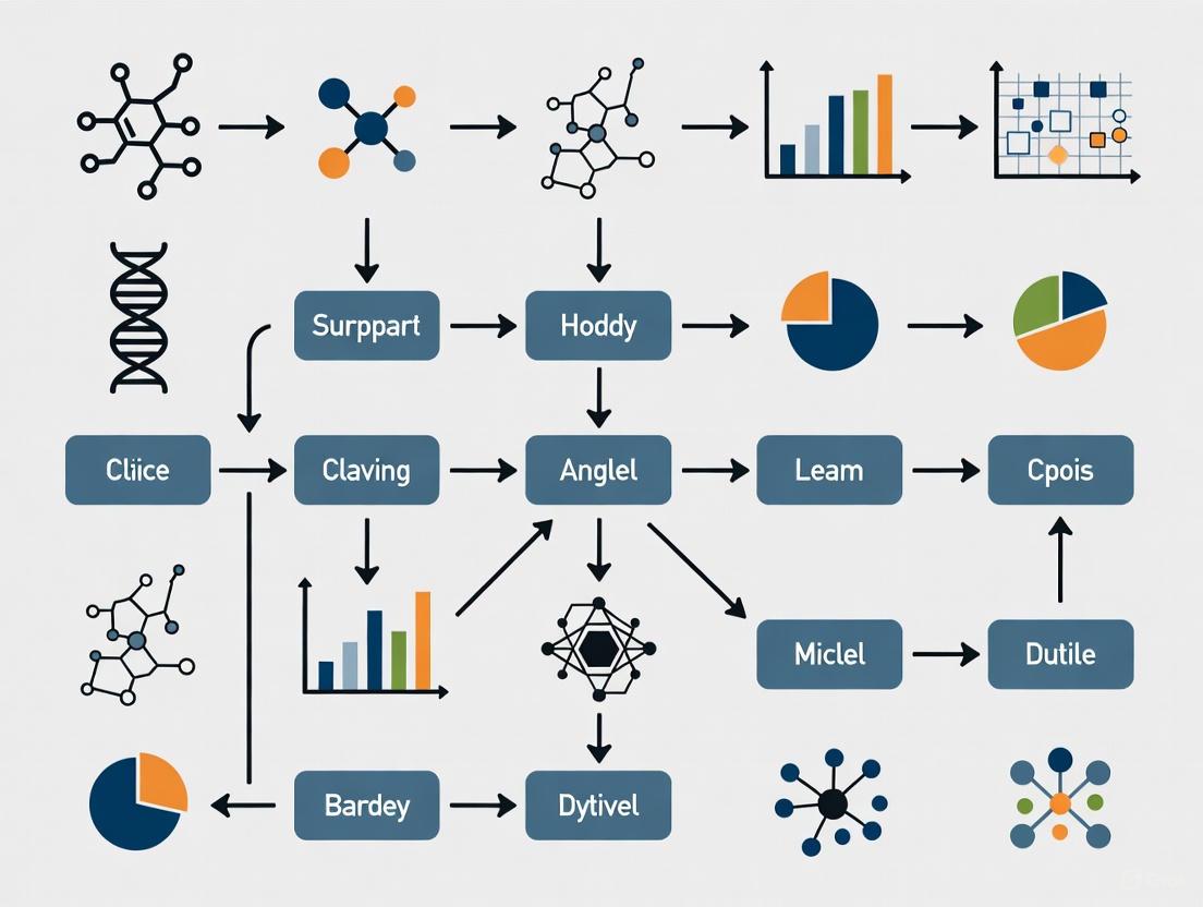
The following diagram illustrates the complete geometric morphometrics workflow from raw data to statistical analysis:

Critical Steps in Detail:

• Generalized Procrustes Analysis (GPA)

  • Translate all configurations to a common origin (usually the centroid)
  • Scale configurations to unit centroid size
  • Rotate configurations to minimize Procrustes distances
  • Iterate until convergence to obtain the consensus configuration

• Shape Variable Extraction

  • Procrustes coordinates represent shape variables after GPA
  • Centroid size (square root of sum of squared distances from landmarks to centroid) serves as size measure
  • Residuals from consensus represent individual shape variation

• Statistical Analysis

  • Principal Component Analysis (PCA): Identifies major axes of shape variation
  • Canonical Variate Analysis (CVA): Maximizes separation among pre-defined groups
  • Regression: Analyzes allometry (shape-size relationships)
  • Modularity/Integration Tests: Examines covariation among anatomical regions

Symmetry Analysis Protocol

Many biological structures exhibit symmetrical organization, requiring specialized analytical approaches. The protocol for symmetry analysis involves:

• Symmetry Definition: Classify symmetry type (bilateral, rotational, translational)
• Landmark Configuration: Assign landmarks to symmetry components
• Procrustes ANOVA: Partition variance into symmetric and asymmetric components
• Biological Interpretation: Relate symmetric and asymmetric variation to developmental, genetic, or environmental factors

For bilaterally symmetric structures, the approach separates variation into:

• Symmetric Component: Differences among individuals
• Asymmetric Component: Differences between sides within individuals (fluctuating asymmetry, directional asymmetry, antisymmetry)

Integration with Machine Learning for Classification

Machine Learning Approaches in Morphometrics

The integration of machine learning (ML) with geometric morphometrics has created powerful frameworks for taxonomic classification and morphological pattern recognition. Recent advances demonstrate several promising approaches:

Functional Data Geometric Morphometrics (FDGM) This innovative approach converts discrete landmark data into continuous curves represented as linear combinations of basis functions [3]. FDGM has demonstrated superior performance in classifying shrew species based on craniodental morphology, outperforming classical GM approaches when combined with machine learning classifiers such as Support Vector Machines and Random Forests [3].

Deep Learning with Convolutional Neural Networks (CNNs) CNNs applied directly to specimen images have shown remarkable performance in classification tasks. In archaeobotanical studies, CNNs outperformed traditional GM methods for seed classification, demonstrating higher accuracy in distinguishing wild from domestic species [4]. This approach leverages automated feature detection rather than relying on manually placed landmarks.

Traditional ML Classifiers with Shape Data Standard machine learning algorithms (Naïve Bayes, SVM, Random Forest, Generalized Linear Models) can be applied to Procrustes shape coordinates or principal component scores derived from GM analysis [3]. This hybrid approach maintains the biological interpretability of GM while leveraging the classification power of ML.

Comparative Performance of GM and ML Methods

Table 3: Performance Comparison of Geometric Morphometrics and Machine Learning Methods

Method	Accuracy Range	Data Requirements	Interpretability	Best Application Context
Traditional GM with Linear Discriminant Analysis	70-85%	20-50 specimens per group	High	Well-defined groups with clear morphological differences
Functional Data GM with ML	85-95% [3]	30+ specimens per group	Moderate	Complex shapes with subtle interspecific variation
Convolutional Neural Networks (CNNs)	>90% [4]	Large datasets (hundreds to thousands)	Low	High-throughput classification without landmark identification
Geometric Morphometrics with Random Forest	80-90%	50+ specimens per group	Moderate	Complex classification problems with multiple groups

The choice between methods depends on research goals: traditional GM provides greater biological interpretability, while ML approaches often achieve higher classification accuracy, particularly for complex morphological patterns [4].

Essential Research Tools and Reagents

Table 4: Research Toolkit for Geometric Morphometric Studies

Tool Category	Specific Tools/Software	Primary Function	Application Context
Imaging Equipment	Micro-CT scanners, Surface laser scanners, Digital microscopes	3D/2D specimen digitization	Data acquisition across scales
Landmark Digitization	TPS Dig2, ImageJ, Landmark Editor	Precise landmark coordinate collection	Initial data collection
Statistical Analysis	R (geomorph, Morpho), MorphoJ, PAST	GM-specific statistical analyses	Shape analysis and hypothesis testing
Machine Learning Integration	R (caret, randomForest), Python (scikit-learn, TensorFlow)	Advanced classification algorithms	Pattern recognition and prediction
Visualization	R (rgl, ggplot2), Paraview, Meshlab	3D shape visualization and rendering	Results communication

Integrated GM-ML Workflow for Classification Research

The following diagram illustrates a modern integrated workflow combining geometric morphometrics and machine learning for classification research:

This integrated framework leverages the strengths of both approaches: GM provides biological interpretability and visualization capabilities, while ML enhances classification performance and pattern recognition. The workflow can be adapted based on research questions, with the GM pathway preferred when understanding specific morphological changes is essential, and the direct ML pathway suitable for high-throughput classification tasks.

Application Notes and Implementation Guidelines

Protocol Optimization for Specific Research Contexts

Taxonomic Classification Studies For distinguishing closely related species, combine high-density semilandmarks with functional data analysis approaches [3]. The dorsal craniodental view has proven particularly informative for shrew species classification. Implement cross-validation procedures to avoid overfitting, especially with limited sample sizes.

Paleontological Applications When working with fragmentary fossil material, utilize template-based semilandmark methods to reconstruct missing regions [2]. Machine learning approaches are particularly valuable for identifying subtle morphological patterns indicative of domestication or environmental adaptations in archaeobotanical remains [4].

Developmental and Evolutionary Studies For analyzing symmetry and asymmetry in evolutionary developmental contexts, implement the Procrustes ANOVA framework to separate directional asymmetry, fluctuating asymmetry, and antisymmetry components [1]. This approach provides insights into developmental stability and canalization.

Data Quality Assurance and Validation

Landmark Reliability Assessment

• Conduct multiple digitization sessions to calculate measurement error
• Use intraclass correlation coefficients to quantify repeatability
• Implement Procrustes ANOVA to partition variance components

Model Validation Protocols

• Apply k-fold cross-validation for machine learning models
• Use holdout test sets never exposed during model training
• Calculate sensitivity, specificity, and balanced accuracy metrics
• Generate confusion matrices to identify systematic misclassifications

Future Directions and Emerging Methodologies

The field continues to evolve with several promising developments:

• Deep learning integration with 3D landmark data for improved classification accuracy
• Automated landmark placement using neural networks to reduce digitization time
• Multimodal data fusion combining geometric morphometrics with genetic, ecological, and functional data
• Open science frameworks enhancing reproducibility through shared data and code protocols [5]

Geometric morphometrics, particularly when integrated with machine learning, provides a powerful quantitative framework for addressing fundamental questions in evolutionary biology, systematics, and functional morphology. By following these standardized protocols and leveraging the appropriate tools, researchers can maximize the insights gained from morphological data while ensuring reproducibility and statistical rigor.

The quantitative analysis of shape, or morphometrics, has undergone a revolutionary transformation with the advent of geometric morphometrics (GM), which enables researchers to capture and analyze the complete geometry of anatomical structures rather than relying on simple linear measurements. This paradigm shift has created unprecedented opportunities across biological, medical, and materials sciences—from classifying insect species for agricultural biosecurity to assessing nutritional status in children and characterizing electro-chemical interfaces in energy materials [6] [7] [8]. However, as morphological datasets grow in dimensionality and complexity, traditional statistical methods like Principal Component Analysis (PCA) and Linear Discriminant Analysis (LDA) face fundamental limitations in capturing the intricate, non-linear patterns inherent in biological and material structures.

PCA, while invaluable for exploratory data analysis and dimensionality reduction, operates on the fundamental assumption that the most informative directions in data space are linear combinations of the original variables that maximize variance [9] [10]. This linearity assumption proves problematic when analyzing complex morphological structures where shape variation follows curved manifolds rather than straight lines. Similarly, LDA, despite its supervised nature that makes it powerful for classification tasks, seeks linear boundaries between predefined classes and assumes normal data distribution and equal class covariances [9] [10]. These mathematical presuppositions rarely hold true for real-world morphological data, where allometric growth patterns, ecological adaptations, and evolutionary constraints create complex non-linear relationships.

The limitations of these traditional approaches become particularly evident in high-stakes applications such as medical diagnostics, species identification with quarantine implications, or development of functional materials, where accurate classification directly impacts health outcomes, economic decisions, and scientific advancement [6] [8] [11]. This application note examines these limitations through both theoretical and practical lenses, provides detailed protocols for implementing advanced machine learning alternatives, and offers a strategic framework for selecting appropriate analytical pathways based on specific research questions and data characteristics.

Critical Limitations of PCA and LDA for Morphological Data Analysis

The Linearity Constraint in Non-Linear Morphological Spaces

The most fundamental limitation of both PCA and LDA lies in their inherent linearity assumption, which directly contradicts the non-linear nature of most morphological phenomena. Biological structures develop and evolve along curved trajectories, with shape changes often following complex allometric patterns where form changes disproportionately with size [9]. When researchers apply PCA to such data, the resulting principal components may effectively capture variance but fail to represent the true underlying biological or physical structure. For instance, in taxonomic studies of leaf-footed bugs (Acanthocephala species), PCA of pronotum shapes accounted for 67% of total shape variation but still resulted in morphological overlaps between closely related species, limiting definitive classification [11].

The linearity problem becomes even more pronounced with LDA, which constructs linear decision boundaries between classes. In morphological datasets with complex class distributions, these straight boundaries inevitably misclassify specimens that fall in the curved regions between class centroids. This limitation was evident in electrochemical impedance spectroscopy data analysis, where LDA's performance for classifying equivalent circuits "crucially depends on slow electrochemical processes" and showed inferior performance compared to non-linear methods [8]. The algorithm's struggle to capture the complex, frequency-dependent processes at electrode-electrolyte interfaces highlights how physical and biological phenomena often inhabit spaces that cannot be adequately partitioned with linear hyperplanes.

The Curse of Dimensionality and Data Sparsity

Morphometric studies frequently generate high-dimensional data, particularly when using landmark-based approaches with numerous coordinates or outline-based methods with hundreds of semilandmarks. In these high-dimensional spaces, PCA and LDA face the "curse of dimensionality," where data becomes increasingly sparse as dimensions grow, fundamentally undermining statistical reliability [9] [10]. The data sparsity problem means that the number of required training examples grows exponentially with each additional dimension to maintain the same coverage density—a requirement rarely feasible in morphological studies where sample collection is often expensive, time-consuming, or limited by rarity.

This dimensionality challenge manifests practically in multiple ways. PCA components become increasingly unstable with high dimension-to-sample size ratios, with the direction of variance captured by each principal component shifting substantially with the addition of new specimens [9]. For LDA, the covariance matrix estimation becomes numerically unstable when the number of features approaches the number of samples, leading to overfitted models that fail to generalize to new data. Research on roselle (Hibiscus sabdariffa L.) morphological traits demonstrated that machine learning models like Random Forest significantly outperformed traditional methods in capturing non-linear genotype-by-environment interactions, achieving R² values of 0.84 compared to poorer performance with linear models [12]. This performance gap underscores how linear methods struggle with the high-dimensional, complex relationships characteristic of morphological datasets.

Sensitivity to Statistical Assumptions and Data Artifacts

Both PCA and LDA carry stringent statistical assumptions that morphological data frequently violate. LDA assumes multivariate normal distributions within each class, equal covariance matrices across classes, and absence of multicollinearity—conditions rarely satisfied in morphological studies where sampling is often unbalanced and covariates are intrinsically correlated [9] [10]. PCA, while less assumption-bound, remains highly sensitive to data scaling, outliers, and missing values, which are common challenges in morphological research involving natural variation or imperfect preservation.

The practical consequences of these statistical limitations are evident across multiple domains. In geometric morphometric approaches for classifying children's nutritional status, researchers noted significant challenges with out-of-sample classification using traditional GM workflows based on Procrustes alignment and linear discrimination [6]. The requirement for a new global alignment for each new specimen introduced artifacts and dependencies on template selection, complicating real-world deployment. Similarly, in urban form analysis, PCA could only capture linear variance in data, failing to identify complex morphological patterns that non-linear methods like UMAP successfully revealed [13]. These case studies highlight how the theoretical foundations of traditional statistical methods constrain their practical utility for complex morphological data.

Table 1: Comparative Limitations of PCA and LDA for Morphological Data Analysis

Limitation Aspect	Impact on PCA	Impact on LDA	Example from Literature
Linearity Assumption	Fails to capture curved manifolds and allometric trajectories	Creates suboptimal linear boundaries between non-linearly separable classes	Urban form analysis required UMAP to reveal non-linear patterns [13]
High-Dimensional Data	Components become unstable with more dimensions than samples	Covariance matrix estimation fails, leading to overfitting	Roselle plant morphology better analyzed with Random Forest (R²=0.84) [12]
Statistical Assumptions	Sensitive to outliers, scaling, and missing data	Requires multivariate normality and equal covariances	EIS data classification required 1D-CNN to handle complex patterns [8]
Class Imbalance	Not directly applicable (unsupervised)	Performance degrades with unbalanced class sizes	Insect identification showed morphological overlaps in closely related species [11]
Interpretability	Components may not correspond to biologically meaningful axes	Directions maximize separation but may not reflect causal factors	Nutritional assessment from arm shapes required specialized alignment [6]

Advanced Machine Learning Approaches for Morphological Data

Non-Linear Manifold Learning Techniques

Non-linear dimensionality reduction techniques address the fundamental linearity constraint of PCA by explicitly modeling the curved manifolds upon which morphological data naturally resides. Algorithms such as t-Distributed Stochastic Neighbor Embedding (t-SNE) and Uniform Manifold Approximation and Projection (UMAP) have demonstrated remarkable success in preserving both local and global topological structures in complex morphological datasets [9] [13]. These methods operate on different principles than PCA—rather than maximizing variance, they preserve neighborhood relationships, enabling them to unfold curved morphological spaces into lower-dimensional representations that maintain meaningful relationships between specimens.

The practical advantages of these non-linear approaches are particularly evident in visualization and exploratory analysis of morphological data. In urban form studies, researchers found that UMAP combined with BIRCH clustering successfully identified 14 distinct urban form types organized into five families with similar characteristics across the metropolitan area of Thessaloniki, Greece [13]. The non-linear embedding captured complex multi-scale morphological patterns that PCA failed to reveal, enabling more nuanced understanding of urban development patterns. Similarly, in single-cell RNA sequencing data (a form of molecular morphology), t-SNE has become the standard for visualizing high-dimensional gene expression patterns, allowing researchers to identify distinct cell types and states based on their transcriptional profiles [9]. These successes across domains highlight how abandoning the linearity constraint enables more faithful representation of complex morphological spaces.

Deep Learning Architectures for Representation Learning

Deep learning methods, particularly autoencoders and convolutional neural networks (CNNs), offer powerful alternatives for morphological data analysis by learning hierarchical representations directly from raw data without relying on pre-specified features or linear transformations. Autoencoders learn to compress high-dimensional morphological data into lower-dimensional latent spaces through encoder-decoder architectures, typically outperforming PCA in reconstruction accuracy and preservation of semantically meaningful features [9] [10]. Variational autoencoders (VAEs) extend this approach by learning probabilistic latent spaces that enable generative sampling and interpolation between morphological forms.

CNNs have revolutionized image-based morphological analysis, automatically learning relevant features from pixel data without requiring manual landmark annotation. In astrophysics, the Spherinator project employs a variational autoencoder with convolutional neural networks to create an explorable 2D representation of simulated galaxy images, enabling morphological classification at unprecedented scale [14]. Similarly, in electrochemical research, 1D-CNNs achieved approximately 86% accuracy in classifying equivalent circuits from impedance spectroscopy data, significantly outperforming linear methods and providing insights into the critical frequency ranges that drive classification decisions [8]. These deep learning approaches demonstrate particular strength when applied to large, complex morphological datasets where manual feature engineering becomes impractical and linear approximations fail to capture meaningful patterns.

Ensemble and Hybrid Approaches

Ensemble methods like Random Forest and hybrid approaches that combine multiple algorithms offer robust alternatives for morphological classification tasks that challenge traditional methods. Random Forest operates by constructing multiple decision trees during training and outputting the mode of classes (classification) or mean prediction (regression) of the individual trees, effectively handling non-linear relationships and high-dimensional data without succumbing to overfitting as readily as single models [12]. Its inherent feature importance measures also provide interpretability missing from many deep learning approaches.

The integration of machine learning with multi-objective optimization algorithms represents a particularly powerful paradigm for morphological analysis. In roselle plant research, combining Random Forest with the Non-dominated Sorting Genetic Algorithm II (NSGA-II) enabled researchers to simultaneously optimize multiple conflicting morphological traits—branch number, growth period, boll number, and seed number—identifying optimal genotype and planting date combinations that would be impossible to discover with traditional methods [12]. Similarly, hybrid workflows that combine non-linear dimensionality reduction with specialized clustering algorithms, such as the UMAP + BIRCH pipeline used in urban form analysis, offer scalable solutions for detecting coherent morphological types in large, high-dimensional datasets [13]. These integrated approaches demonstrate how moving beyond standalone statistical methods enables more comprehensive morphological analysis and optimization.

Table 2: Machine Learning Alternatives to PCA and LDA for Morphological Data

Method	Key Advantages	Ideal Use Cases	Implementation Considerations
t-SNE	Preserves local structure and reveals clusters	Visualization of high-dimensional data, exploratory analysis	Perplexity parameter sensitive; cluster sizes not meaningful [9] [10]
UMAP	Better preservation of global structure than t-SNE	Large-scale morphological datasets, preprocessing for clustering	More scalable than t-SNE; preserves more global structure [13]
Autoencoders	Learns non-linear representations; generative capability	Complex feature extraction, data compression, anomaly detection	Requires more data and tuning; variational versions enable sampling [9] [14]
Random Forest	Handles non-linearity and high dimensionality; robust to outliers	Classification and regression with complex feature interactions	Provides feature importance; less interpretable than linear models [12]
1D/2D-CNNs	Automatically learns relevant features from raw data	Image-based morphology, spectral data, time-series morphology	Requires substantial data; minimal preprocessing needed [8]

Experimental Protocols for Advanced Morphological Analysis

Protocol 1: Dimensionality Reduction with UMAP

Principle: Uniform Manifold Approximation and Projection (UMAP) constructs a high-dimensional graph representation of data then optimizes a low-dimensional layout to preserve as much of the topological structure as possible [13]. Unlike PCA, UMAP makes no linearity assumptions and can capture complex non-linear relationships in morphological data.

Step-by-Step Workflow:

• Data Preparation: Standardize all morphological features (landmark coordinates, linear measurements, or outline data) using z-score normalization to ensure equal contribution to the manifold learning process.
• Parameter Selection: Set the number of neighbors (typically 15-50) to balance local versus global structure preservation. Higher values emphasize global structure.
• Minimum Distance Tuning: Adjust the minimum distance parameter (typically 0.1-0.5) to control how clustered the embedding appears. Lower values result in tighter clusters.
• Manifold Construction: Compute the UMAP embedding using the standardized data and selected parameters.
• Validation: Assess embedding quality through downstream tasks (clustering accuracy, classification performance) or qualitative assessment of known morphological groupings.

Applications: This protocol has been successfully applied to urban form analysis, where UMAP reduced 17 multi-scale morphological indicators to a lower-dimensional space before clustering with BIRCH, revealing 14 distinct urban form types with geographical coherence [13].

Protocol 2: Morphological Classification with 1D-CNN

Principle: 1D Convolutional Neural Networks (CNNs) learn hierarchical features directly from raw data sequences, making them ideal for classifying morphological data represented as landmark coordinates, outline points, or spectral measurements [8].

Step-by-Step Workflow:

• Data Representation: Format morphological data as 1D sequences, preserving the natural ordering of landmarks or measurements.
• Architecture Design: Construct a 1D-CNN with alternating convolutional and pooling layers to learn features at multiple scales, followed by fully connected layers for classification.
• Model Training: Train the network using appropriate loss functions (categorical cross-entropy for classification) with regularization (dropout, batch normalization) to prevent overfitting.
• Interpretation: Apply explainable AI techniques like SHAP analysis to identify which morphological features most influence classification decisions.
• Validation: Evaluate performance using hold-out test sets or cross-validation, reporting accuracy, F1-score, and confusion matrices.

Applications: This approach achieved approximately 86% accuracy in classifying equivalent circuits from electrochemical impedance spectroscopy data, significantly outperforming traditional methods and providing insights into the critical frequency ranges that drive classification decisions [8].

Protocol 3: Multi-Objective Optimization with ML and NSGA-II

Principle: Integrating machine learning models with multi-objective evolutionary algorithms enables simultaneous optimization of multiple, potentially conflicting morphological traits [12].

Step-by-Step Workflow:

• Data Collection: Assemble morphological measurements across multiple traits of interest from specimens representing different genotypes, treatments, or conditions.
• Model Training: Develop predictive models (Random Forest recommended) for each morphological trait based on input parameters (genotype, environmental conditions).
• Optimization Setup: Define objective functions for each trait to be optimized, specifying direction (maximize/minimize) and constraints.
• NSGA-II Execution: Implement the Non-dominated Sorting Genetic Algorithm II to identify Pareto-optimal solutions representing the best trade-offs between objectives.
• Validation: Experimentally verify predicted optima and refine models iteratively with additional data.

Applications: This protocol successfully optimized roselle plant morphology, identifying that the Qaleganj genotype planted on May 5 produced optimal values for branch number (26), growth period (176 days), boll number (116), and seed numbers (1517) per plant [12].

Table 3: Essential Software and Computational Tools for Morphological Machine Learning

Tool/Platform	Primary Function	Application in Morphological Research	Implementation Considerations
MorphoJ [11]	Geometric morphometrics analysis	Generalized Procrustes analysis, PCA, discriminant analysis	Specialized for landmark data; user-friendly interface
Scikit-learn [12]	Machine learning in Python	PCA, LDA, Random Forest, and other ML algorithms	Extensive documentation; integration with scientific Python stack
UMAP [13]	Non-linear dimensionality reduction	Visualization and preprocessing of complex morphological data	Parameters significantly affect results; requires tuning
TensorFlow/PyTorch [14]	Deep learning frameworks	Autoencoders, CNNs for complex morphological pattern recognition	Steeper learning curve; requires GPU for large datasets
StreamFlow/Flyte [14]	Workflow orchestration	Reproducible pipelines for large-scale morphological analysis	StreamFlow for HPC clusters; Flyte for cloud-native environments

The limitations of PCA and LDA for complex morphological data necessitate a more nuanced, problem-driven approach to analytical method selection. Through the case studies and protocols presented herein, a clear framework emerges for matching methodological approach to research question. For visualization and exploration of unknown morphological spaces, non-linear dimensionality reduction techniques like UMAP provide superior insights compared to PCA. For classification tasks with complex decision boundaries, deep learning approaches like 1D-CNNs outperform LDA while offering interpretability through explainable AI techniques. Most powerfully, integrated machine learning and optimization frameworks enable not just description but active optimization of morphological traits.

The progression beyond traditional statistics does not render methods like PCA and LDA obsolete—they remain valuable for initial data exploration, baseline comparisons, and applications where linear approximations suffice. However, researchers working with complex morphological data must expand their analytical toolkit to include the non-linear, ensemble, and deep learning approaches detailed in this application note. By doing so, they can overcome the fundamental constraints of linear methods and uncover richer, more meaningful patterns in morphological data—advancing fields as diverse as taxonomy, materials science, biomedical research, and beyond.

Functional Data Geometric Morphometrics (FDGM) represents a paradigm shift in shape analysis, moving beyond discrete landmark points to model biological forms as continuous mathematical curves. This innovative approach combines the statistical rigor of Functional Data Analysis (FDA) with the established principles of Geometric Morphometrics (GM), enabling researchers to capture subtle shape variations that traditional methods might miss [3]. By treating entire shapes as functions, FDGM opens new possibilities for analyzing complex biological structures in evolutionary biology, taxonomy, and paleontology.

The fundamental innovation of FDGM lies in its treatment of landmark data not as isolated points, but as points interconnected to form continuous curves. These curves are then represented as linear combinations of basis functions, allowing for analysis of shape variation across the entire form rather than just at predetermined landmark locations [3]. This approach is particularly valuable for studying structures where biologically significant shape variations occur between traditional landmarks, providing a more comprehensive understanding of morphological diversity.

Core Concepts of FDGM

From Discrete Landmarks to Continuous Functions

Traditional geometric morphometrics relies on the precise placement of anatomical landmarks - discrete points that correspond biologically across specimens [3]. While powerful, this approach inherently limits analysis to specific, predetermined locations, potentially missing meaningful shape information that occurs between landmarks.

FDGM addresses this limitation through a conceptual and mathematical transformation:

• Curve Conversion: 2D landmark data is converted into continuous curves through interpolation techniques
• Basis Function Representation: These continuous curves are represented as linear combinations of mathematical basis functions
• Functional Space Analysis: Statistical analyses are performed within the functional space rather than on discrete point coordinates [3]

This functional representation enables researchers to analyze shape variation as a continuous phenomenon across the entire structure, rather than being constrained to discrete measurement points.

Mathematical Foundation

The mathematical framework of FDGM builds upon functional data analysis principles. Each shape is represented as a function:

[f(t) = \sum{k=1}^{K} ck \phi_k(t)]

where (\phik(t)) are basis functions (e.g., Fourier basis or B-splines), (ck) are coefficients, and (t) represents the spatial domain [3]. This representation allows for the application of functional versions of standard statistical methods, including functional principal component analysis (FPCA) and functional linear discriminant analysis.

A critical step in FDGM involves curve registration or functional alignment to ensure that corresponding geometric features (peaks, valleys) are properly aligned across specimens [3]. This process accounts for non-rigid deformations and complex shape changes that may not be captured by traditional Procrustes alignment alone.

Comparative Framework: FDGM vs. Traditional Approaches

Methodological Comparison

Table 1: Comparison between Traditional GM and FDGM Approaches

Feature	Traditional GM	FDGM
Data Representation	Discrete landmark coordinates	Continuous curves/functions
Shape Information	Limited to landmark positions	Captures between-landmark variation
Alignment Method	Generalized Procrustes Analysis (GPA)	GPA + Functional alignment/curve registration
Statistical Framework	Multivariate statistics	Functional data analysis
Landmark Requirement	Requires exact correspondence	More flexible with landmark correspondence

Performance Advantages

Recent studies have demonstrated significant advantages of FDGM over traditional approaches:

• Enhanced Sensitivity: FDGM shows improved sensitivity to subtle shape variations, particularly for species with minor morphological distinctions [3]
• Superior Classification Accuracy: In shrew craniodental classification, FDGM outperformed traditional GM, with the dorsal view providing best distinction between species [3]
• Comprehensive Shape Capture: The continuous curve approach captures shape information between traditional landmarks, providing more complete morphological characterization [3]

Extension to three-dimensional data further enhances these advantages. Recent innovations incorporate square-root velocity function (SRVF) and arc-length parameterization for 3D morphometric data, enabling analysis of complex surfaces and volumes while preserving geometric properties [15].

Application Notes: Implementation Protocols

Standard FDGM Protocol for 2D Data

Table 2: Step-by-Step FDGM Protocol for 2D Shape Classification

Step	Procedure	Tools/Packages	Key Parameters
1. Data Acquisition	Capture 2D images of specimens under standardized conditions	Digital camera with fixed setup	Consistent orientation, scale, and resolution
2. Landmark Digitization	Place homologous landmarks on all specimens	TpsDig2, MorphoJ [16]	13-15 landmarks typically sufficient [16]
3. Curve Conversion	Convert landmark coordinates to continuous curves	Custom R/Python scripts	Fourier or B-spline basis functions
4. Functional Alignment	Align curves to account for non-rigid deformations	FDA packages (R/Python)	Landmark-based registration
5. Shape Analysis	Apply functional PCA and discriminant analysis	Functional data analysis packages	Number of principal components
6. Machine Learning Integration	Implement classifiers using shape features	Naïve Bayes, SVM, Random Forest, GLM [3]	Cross-validation for parameter tuning

Advanced 3D FDGM Protocol

For three-dimensional data, the protocol extends to incorporate recent methodological innovations:

• Data Acquisition: 3D scanning or photogrammetry (e.g., Structure-from-Motion) [17]
• Preprocessing: Point cloud classification using geometric features and RGB values [17]
• Functional Representation: Apply SRVF and arc-length parameterization [15]
• Analysis Pipelines: Implement multiple approaches including FDM, arc-FDM, soft-SRV-FDM, and elastic-SRV-FDM [15]

Machine Learning Integration

Classification Framework

The integration of machine learning with FDGM significantly enhances classification performance across biological applications:

• Feature Extraction: Functional principal component scores serve as input features for classifiers [3]
• Algorithm Selection: Multiple algorithms including Naïve Bayes, Support Vector Machine, Random Forest, and Generalized Linear Models have been successfully applied [3]
• Performance Validation: Cross-validation and independent test sets ensure robust performance assessment

In shrew species classification, the combination of FDGM with machine learning achieved superior classification accuracy compared to traditional GM approaches, with the dorsal craniodental view providing the most discriminatory power [3].

Comparative Performance

Table 3: Machine Learning Classification Performance with Morphometric Approaches

Application Domain	Traditional GM Accuracy	FDGM Accuracy	Best Performing Classifier
Shrew Craniodental Classification	Lower than FDGM [3]	Superior performance [3]	Varies by view (dorsal best) [3]
Deep-Sea Coral/Sponge Classification	N/A	N/A	Random Forest (84.5% accuracy) [17]
Seed Domestication Classification	Outperformed by CNN [4]	N/A	Convolutional Neural Networks [4]
Kangaroo Dietary Classification	Baseline for comparison [15]	Enhanced with FDA innovations [15]	Support Vector Machines [15]

Research Toolkit

Essential Software and Analytical Tools

Table 4: Essential Research Tools for FDGM Implementation

Tool Name	Function	Application Context
TpsDig2 [16]	Landmark digitization	Collecting 2D coordinate data from images
MorphoJ [16]	Geometric morphometrics analysis	Traditional GM and preliminary shape analysis
R FDA Package	Functional data analysis	Implementing FDGM statistical analyses
Python Scikit-learn	Machine learning implementation	Classification algorithms and validation
Custom SRVF Scripts [15]	3D functional analysis	Advanced 3D shape analysis pipelines

Experimental Materials Protocol

For morphological studies employing FDGM:

• Sample Preparation: Standardize specimen orientation and imaging conditions [3]
• Landmark Selection: Choose biologically homologous points covering key morphological features [16]
• Data Quality Control: Implement reproducibility protocols including open data and code sharing [5]
• Validation Sets: Reserve specimens for independent testing of classification models [3]

Visualization and Workflow

FDGM Analytical Workflow: From specimen collection to classification results.

Methodological Comparison: Traditional GM versus FDGM approach.

Functional Data Geometric Morphometrics represents a significant advancement in shape analysis methodology. By modeling biological forms as continuous curves rather than discrete points, FDGM captures more comprehensive shape information and enhances classification performance when integrated with machine learning algorithms.

The future development of FDGM points toward several promising directions:

• Integration with Deep Learning: Combining functional data approaches with convolutional neural networks for enhanced pattern recognition [4]
• Expansion to 3D Data: Application of SRVF and elastic registration methods to three-dimensional morphological data [15]
• Multimodal Data Fusion: Combining shape data with other data types (genetic, ecological) for comprehensive biological analysis
• Reproducibility Frameworks: Addressing current limitations in reproducibility through standardized protocols and open data sharing [5]

As morphological studies continue to evolve, FDGM provides a powerful framework for extracting maximum biological information from shape data, with applications spanning taxonomy, evolutionary biology, ecology, and archaeological science. The integration of this innovative morphological approach with machine learning classification represents a particularly promising pathway for advancing quantitative morphological research.

Why Machine Learning? Addressing Non-Linearities and High-Dimensional Shape Data

The analysis of biological shape is a fundamental endeavor in fields ranging from drug development to evolutionary biology. Geometric Morphometrics (GM) has long been the standard quantitative framework for capturing and analyzing shape variation using landmark coordinates [3]. However, traditional statistical methods often struggle with the inherent complexities of shape data, which is characteristically high-dimensional and may contain complex non-linear relationships [3] [18]. Machine Learning (ML) provides a powerful suite of tools that directly address these challenges, enabling researchers to build more accurate and robust classification models from morphometric data. This document outlines the theoretical rationale for applying ML to GM and provides detailed protocols for its implementation in classification research.

The core challenge lies in the nature of shape data itself. After a Generalized Procrustes Analysis (GPA), which aligns landmark configurations by removing differences in position, orientation, and scale, the resulting data exists in a high-dimensional space [3]. When analyzing complex structures with many landmarks, the number of dimensions can easily exceed the number of specimens, a scenario where traditional statistical models are prone to overfitting and lose their ability to generalize to new data [18] [19]. Furthermore, the biological relationships underpinning shape variation—such as allometric growth patterns or adaptations to ecological niches—are often non-linear. While methods like Principal Component Analysis (PCA) can reduce dimensionality, they are inherently linear and may fail to capture these more complex patterns [3] [20].

Machine learning models are exceptionally well-suited to this context. They can natively handle high-dimensional input spaces and, through the use of non-linear activation functions (e.g., ReLU, Sigmoid) or kernel methods, learn intricate decision boundaries that linear models cannot [21]. This allows ML to detect subtle, data-driven patterns in shape, thereby improving classification accuracy for tasks such as taxonomic identification, morphological response to treatment, or diagnostic screening [5] [4] [22].

Quantitative Comparisons: Machine Learning vs. Traditional Morphometrics

The superiority of ML approaches, particularly deep learning, is demonstrated by their performance in direct comparative studies. The following tables summarize key findings from recent research.

Table 1: Comparative Performance of GM and ML in Species Classification

Study Subject	Method	Key Performance Metric	Result	Reference
Shrew Crania (3 species)	Functional Data GM (FDGM) + Machine Learning	Classification Accuracy	Favored FDGM; Dorsal view was best	[3]
Archaeobotanical Seeds	Geometric Morphometrics (GMM)	Classification Accuracy	Outperformed by CNN	[4]
Archaeobotanical Seeds	Convolutional Neural Network (CNN)	Classification Accuracy	Superior to GMM	[4]
Cut Marks (Tool Type)	Geometric Morphometrics + Machine Learning	Identification of tool material (flint vs. metal)	Successfully identified flint tools on Iron Age site	[22]

Table 2: Machine Learning Algorithms for High-Dimensional and Small Data Challenges

Algorithm Category	Example Algorithms	Strengths	Ideal Use Case in Morphometrics
Traditional ML	Support Vector Machine (SVM), Random Forest (RF), Naïve Bayes	Effective in high-dimensional spaces; Less prone to overfitting with small data than deep learning	Initial classification models with limited sample size [3] [19]
Deep Learning	Convolutional Neural Networks (CNNs)	Automatically learns relevant features; State-of-the-art for image-based classification	Direct classification from images, bypassing landmarking [5] [4]
Dimensionality Reduction	PCA, t-SNE, UMAP, Autoencoders	Reduces data complexity; Aids in visualization and model performance	Pre-processing step for high-dimensional landmark data [18] [23]

Experimental Protocols

This section provides a detailed workflow for applying machine learning to geometric morphometric data, from data acquisition to model interpretation.

Protocol 1: A Standard Workflow for Landmark-Based ML Classification

Application Note: This protocol is designed for classification tasks (e.g., species, genotypes, treatment groups) when data is collected as 2D or 3D landmarks.

Materials and Reagents:

• Specimens (e.g., skulls, seeds, medical images)
• Imaging equipment (e.g., microscope with camera, micro-CT scanner)
• Software for digitizing landmarks (e.g., MorphoJ, tpsDig2)
• Computing environment with programming capabilities (e.g., R, Python)

Procedure:

• Data Acquisition:
  • Image Capture: Standardize imaging conditions (orientation, scale, lighting) to minimize non-biological variance. For the shrew crania study, three standardized views (dorsal, jaw, lateral) were used [3].
  • Landmark Digitization: Identify and digitize homologous anatomical landmarks across all specimens. The number of landmarks should be sufficient to capture the geometry of the biological structure [3].

• Data Preprocessing:

  • Generalized Procrustes Analysis (GPA): Perform GPA on the raw landmark coordinates to superimpose configurations, removing variation due to translation, rotation, and scale. The resulting Procrustes coordinates represent shape variables for subsequent analysis [3] [22].
  • Training/Test Split: Randomly split the Procrustes coordinates and their associated class labels into a training set (e.g., 70-80%) and a held-out test set (e.g., 20-30%). The test set must only be used for the final evaluation of the model's generalization ability.

• Dimensionality Reduction and Model Training:

  • Principal Component Analysis (PCA): Perform PCA on the Procrustes coordinates from the training set. The principal components (PCs) are new, uncorrelated variables that capture the major axes of shape variance [3] [22].
  • Feature Selection: Use the PC scores as features for the machine learning model. The number of PCs to retain can be determined by a scree plot or by retaining enough PCs to explain a high percentage (e.g., >95%) of the total variance.
  • Model Training: Train a selected machine learning classifier (e.g., SVM, Random Forest, Naïve Bayes) using the PC scores from the training set. Optimize model hyperparameters via cross-validation on the training set only [3].

• Model Evaluation:

  • Prediction: Use the trained model to predict class labels for the held-out test set.
  • Performance Metrics: Calculate accuracy, precision, recall, F1-score, and generate a confusion matrix to evaluate model performance [4].

Protocol 2: Functional Data and Deep Learning Approaches

Application Note: This protocol outlines advanced methods that can capture subtler shape variations, either by treating outlines as continuous functions or by using deep learning to bypass landmark digitization.

Procedure:

• Functional Data Geometric Morphometrics (FDGM):
  • Curve Representation: Convert discrete 2D landmark data into continuous curves using mathematical basis functions (e.g., B-splines) [3].
  • Analysis: Analyze the resulting functional data using methods like functional PCA. This approach can be more sensitive to shape variations that occur between traditional landmarks [3].
  • Machine Learning Integration: As with standard GM, the scores from functional PCA can be used as features in standard machine learning classifiers to improve classification performance [3].

• Deep Learning with Convolutional Neural Networks (CNNs):
  • Input Data: Use the standardized raw images as direct input to the model, bypassing the landmark digitization step entirely [4].
  • Model Architecture: Employ a CNN architecture (e.g., VGG, ResNet). The convolutional layers will automatically learn discriminative features directly from the pixel data.
  • Training: Train the CNN on the labeled images. Techniques like transfer learning (using a pre-trained model) and data augmentation (rotating, flipping images) can be highly effective, especially with smaller datasets [5] [4].
  • Comparison: This approach has been shown to outperform GMM in tasks like seed classification, as it leverages the full image information rather than a pre-defined set of points [4].

The following workflow diagram illustrates the two primary pathways for applying machine learning to shape data.

The Scientist's Toolkit: Research Reagent Solutions

Table 3: Essential Materials and Software for Morphometric Machine Learning

Item Name	Function/Application	Specification Notes
Structured-Light 3D Scanner (e.g., DAVID SLS-2)	High-resolution 3D model generation for detailed shape capture.	Used for creating 3D models of bones/tools for cross-sectional analysis [22].
Generalised Procrustes Analysis (GPA)	The foundational statistical procedure for aligning landmark configurations and extracting pure "shape" variables.	A critical pre-processing step before any shape analysis [3] [22].
R Statistical Software	Primary environment for conducting Geometric Morphometrics and traditional statistical analysis.	Key packages: Momocs for GMM, geomorph for GM analysis [4].
Python Programming Language	Primary environment for building and training machine learning and deep learning models.	Key libraries: scikit-learn for SVM/RF, TensorFlow/PyTorch for CNNs, NumPy for data handling [18].
Principal Component Analysis (PCA)	Linear dimensionality reduction technique to transform high-dimensional shape data into a lower-dimensional set of uncorrelated components.	PC scores are used as features for machine learning models to prevent overfitting [3] [18].
Support Vector Machine (SVM)	A powerful classification algorithm effective in high-dimensional spaces, capable of learning non-linear boundaries using kernel functions.	One of several traditional ML models suitable for morphometric classification [3] [19].
Convolutional Neural Network (CNN)	A class of deep neural networks most commonly applied to analyzing visual imagery, capable of automated feature learning.	Outperforms traditional GMM in image-based classification tasks (e.g., seed identification) [5] [4].

The integration of machine learning with geometric morphometrics represents a significant methodological advance for classification research. ML directly addresses the core challenges of morphometric data—its high dimensionality and potential non-linearities—by providing tools that are more flexible and powerful than traditional statistical methods. As demonstrated in studies across biology, archaeology, and paleontology, ML techniques, from SVMs to CNNs, consistently achieve high classification accuracy, uncover subtle morphological patterns, and offer automation potential. The protocols provided herein offer a roadmap for researchers in drug development and other scientific fields to leverage these powerful tools, thereby enhancing the rigor, reproducibility, and scope of their shape-based analyses.

Building the Machine Learning Pipeline for Morphometric Data

In the field of drug discovery and pharmaceutical research, the quantitative analysis of biological shape—or geometric morphometrics—has emerged as a critical tool for understanding phenotypic changes induced by therapeutic compounds or disease states [24]. The high failure rates and exorbitant costs associated with traditional drug development pipelines have intensified the need for more predictive preclinical models and analytical methods [25] [26]. Machine learning (ML) offers powerful capabilities for pattern recognition in complex datasets, but its effectiveness hinges on appropriate data preprocessing and feature engineering [25]. This application note details methodologies for transforming raw morphological data into features suitable for ML-driven classification research, with specific applications for researchers and drug development professionals.

Core Concepts in Morphological Feature Engineering

Procrustes Coordinates: Establishing Biological Homology

Procrustes analysis is a cornerstone of geometric morphometrics, providing a statistical framework for comparing biological shapes by removing non-shape-related variations. The process involves a similarity test for two datasets where each input matrix represents sets of points or vectors (the rows of the matrix) [27].

The Generalized Procrustes Analysis (GPA) standardizes configurations of landmark points through three operations [24] [28]:

• Translation: Configurations are centered around the origin by subtracting centroid coordinates.
• Scaling: Configurations are scaled to unit size, typically achieved by setting (tr(AA^{T}) = 1) [27].
• Rotation: Configurations are rotated to minimize the sum of squared distances between corresponding landmarks, known as the Procrustes distance [27].

The mathematical objective is to minimize (M^{2}=\sum(data1-data2)^{2}), the sum of the squares of the pointwise differences between the two input datasets [27]. This process ensures that shape comparisons focus solely on biologically meaningful variations rather than differences in position, orientation, or size.

Outline Representations: Capturing Continuous Morphology

While landmark-based methods excel when homologous points are available, many biological structures lack clearly defined landmarks or exhibit shape variations between phylogenetically distant species where homology is ambiguous [29]. Outline representations address this limitation by capturing the continuous contour of a structure. Common methodologies include:

• Elliptic Fourier Analysis (EFA): Describes closed contours through Fourier coefficients, effectively capturing smooth outlines [29].
• Landmark-Free Deep Learning: Approaches like Morpho-VAE (Morphological regulated Variational AutoEncoder) use image-based deep learning frameworks to extract morphological features without manual landmark annotations [29]. This method combines unsupervised and supervised learning to reduce dimensionality while focusing on morphologically discriminative features.

Experimental Protocols

Protocol 1: Generalized Procrustes Analysis for Standardization

Application Context: Aligning 3D nasal cavity landmark data to assess olfactory region accessibility for nose-to-brain drug delivery [24].

• Materials and Software:

  • 3D meshes of biological structures (e.g., from CT scans)
  • Software: Viewbox 4.0, R with geomorph package [24]
  • Anatomically defined fixed landmarks and sliding semi-landmarks

• Methodology:

  • Landmark Digitization: Manually place fixed anatomical landmarks on a template model in homologous regions present across all specimens [24].
  • Semi-Landmark Placement: Distribute semi-landmarks across surface patches of the template model. Use Thin Plate Spline (TPS) warping to project these semi-landmarks from the template to each specimen, allowing them to slide tangentially along the surface to minimize bending energy [24].
  • GPA Implementation: Input the raw landmark coordinates (fixed and slid semi-landmarks) into the GPA algorithm to perform:
    • Translation: Center each configuration to its centroid.
    • Scaling: Scale all configurations to a unit centroid size.
    • Rotation: Iteratively rotate configurations to minimize the Procrustes sum of squares [24] [28].
  • Output: The aligned Procrustes coordinates, which represent the shape information free of position, orientation, and size effects, are now ready for subsequent multivariate analysis or as features for machine learning models.

Protocol 2: Landmark-Free Feature Extraction Using Morpho-VAE

Application Context: Classifying primate mandible shapes to understand morphological adaptations without predefined landmarks [29].

• Materials and Software:

  • Sample images of biological structures (e.g., mandibles)
  • Python with deep learning frameworks (e.g., TensorFlow, PyTorch)
  • Morpho-VAE architecture [29]

• Methodology:

  • Image Preprocessing: For 3D objects, generate multiple 2D projections from different angles (e.g., frontal, lateral, superior). Standardize image size and orientation [29].
  • Morpho-VAE Architecture Setup:
    • Configure the VAE module with encoder and decoder networks.
    • Integrate a classifier module that connects to the latent space.
    • Define the combined loss function: (E{total} = (1 - \alpha)E{VAE} + \alpha E{C}), where (E{VAE}) is the VAE loss (reconstruction + regularization), (E_{C}) is the classification loss, and (\alpha) is a hyperparameter (e.g., 0.1) balancing both objectives [29].
  • Model Training:
    • Train the network on the image dataset.
    • The encoder learns to compress input images into a low-dimensional latent space ((\zeta)).
    • The classifier ensures that the latent space captures features discriminative for the labeled classes (e.g., species families) [29].
  • Feature Extraction: Use the trained encoder to transform input images into latent vectors ((\zeta)). These vectors serve as the landmark-free feature representation for downstream machine learning tasks like classification or clustering.

The following diagram illustrates the Morpho-VAE workflow for landmark-free feature extraction:

Comparative Analysis of Feature Engineering Approaches

Table 1: Comparison of Morphological Feature Engineering Techniques

Feature Type	Mathematical Foundation	Data Requirements	Primary Applications in Drug Discovery	Key Advantages	Key Limitations
Procrustes Coordinates	Generalized Procrustes Analysis (GPA) [24] [28]	Anatomically defined landmarks (fixed and sliding semi-landmarks) [24]	- Personalizing nasal drug delivery [24]- Quantifying morphological biomarkers	- Maintains biological homology- Strong statistical theory- Results are interpretable	- Requires expert anatomical knowledge- Limited to structures with definable landmarks
Outline Representations (EFA)	Elliptic Fourier Analysis [29]	Continuous outline coordinates	- Characterizing cell morphology [29]- Analyzing organelle shapes	- Suitable for smooth, complex outlines- Does not require homologous points	- Less effective for structures with sharp angles or internal details- May require many coefficients
Landmark-Free Deep Learning (Morpho-VAE)	Variational Autoencoder (VAE) with classifier integration [29]	2D image projections of 3D structures [29]	- High-throughput phenotypic screening- Classifying tissue morphology in digital pathology	- Fully automated- Captures complex, non-linear shape features- Can impute missing data [29]	- "Black box" nature reduces interpretability- Requires large datasets for training

The Scientist's Toolkit: Essential Research Reagents & Materials

Table 2: Key Reagents and Computational Tools for Morphological Analysis

Item Name	Specification/Function	Application Context
Viewbox 4.0	Software for digitizing landmarks and semi-landmarks, and performing Geometric Morphometric analysis [24].	Precise placement of anatomical landmarks and semi-landmarks on 3D models for Procrustes analysis [24].
R geomorph Package	An R package for performing geometric morphometric shape analysis, including GPA and PCA [24].	Statistical analysis of shape, multivariate regression, and visualization of shape variations.
Sliding Semi-Landmarks	Points placed on curves and surfaces that slide to minimize bending energy, allowing comparison of non-homologous regions [24].	Capturing the geometry of complex biological surfaces and contours between fixed landmarks in 3D studies [24].
Generalized Procrustes Analysis (GPA)	Algorithm that standardizes landmark configurations by removing effects of position, scale, and orientation [24] [28].	The core step in landmark-based morphometrics to isolate pure "shape" information for statistical comparison.
Morpho-VAE Framework	A deep learning architecture combining a Variational Autoencoder (VAE) with a classifier to extract discriminative shape features [29].	Landmark-free, automated feature extraction from 2D image data for classification tasks (e.g., mandible morphology) [29].
ITK-SNAP	Open-source software for semi-automatic segmentation of 3D medical images [24].	Creating 3D surface meshes from CT or MRI scans, which serve as the base for landmarking.

Implementation Workflow for ML-Based Morphometric Classification

The integration of feature engineering with machine learning classification involves a structured pipeline, from data acquisition to model deployment, as visualized below:

This workflow demonstrates two parallel paths for feature extraction—landmark-based and landmark-free—that converge at the machine learning classification stage. This flexible approach allows researchers to select the most appropriate method based on their specific data characteristics and research objectives.

The integration of machine learning (ML) with geometric morphometric (GM) data is transforming biological classification research. By quantifying shape from anatomical landmarks, GM provides a rich, high-dimensional dataset that ML algorithms can leverage for precise taxonomic, ecological, and phenotypic discrimination [3]. This combination is particularly powerful in applications ranging from species classification to nutritional assessment and forensic analysis [6] [30]. The selection of an appropriate algorithm is paramount, as the performance of different ML models can vary significantly based on the data structure, sample size, and research objective.

This article provides a structured comparison of four prominent classification algorithms—Support Vector Machine (SVM), Random Forest (RF), Naïve Bayes (NB), and Generalized Linear Models (GLM)—within the context of geometric morphometrics. We present quantitative performance comparisons from recent studies, detail standardized protocols for implementation, and visualize the analytical workflow to equip researchers with the practical knowledge needed to select and apply the optimal model for their classification tasks.

Performance Comparison in Morphometric Research

Empirical evidence from recent studies provides critical guidance for algorithm selection. The following tables summarize the performance of SVM, RF, NB, and GLM across diverse morphometric classification tasks.

Table 1: Algorithm Performance in Shrew Craniodental Species Classification [3] [31]

Algorithm	Accuracy	Precision	Recall	F1-Score	Notes
Generalized Linear Model (GLM)	95.4%	Not Reported	Not Reported	Not Reported	Best performer with Functional Data GM
Support Vector Machine (SVM)	89.9%	Not Reported	Not Reported	Not Reported	Third best performance
Random Forest (RF)	90.4%	Not Reported	Not Reported	Not Reported	Second best performance
Naïve Bayes (NB)	86.5%	Not Reported	Not Reported	Not Reported	Lowest performance among the four

Table 2: Algorithm Performance in Other Morphometric and Classification Contexts

Study Context	Best Performer	Performance	Other Algorithms	Performance
Fake News Classification [32]	SVM	100% Accuracy	Random Forest	99% Accuracy
			Naïve Bayes	94% Accuracy
Sex Estimation from 3D Tooth Shapes [30]	Random Forest	97.95% Accuracy	Support Vector Machine	70-88% Accuracy
			Artificial Neural Network	58-70% Accuracy
Stingless Bee Species Classification [33]	SVM with SMOTE	AUC: 0.9918, Sensitivity: 0.959	Random Forest with SMOTE	Lower AUC & Sensitivity

Essential Research Toolkit for GM-ML Classification

A successful GM-ML pipeline requires specialized tools and software for data acquisition, processing, and analysis.

Table 3: Key Research Reagents and Software Solutions

Item Name	Function / Application	Specific Example / Note
3D Scanner / Digitizer	Captures high-resolution 3D surface data of specimens.	Lab-based scanners (e.g., inEOS X5) for dental casts [30].
Landmarking Software	Allows precise placement of 2D/3D landmarks on specimens.	3D Slicer [30], MorphoJ [30], Thin Plate Spline (TPS) software [3].
Statistical Shape Analysis Tools	Performs Procrustes alignment and basic statistical shape analysis.	MorphoJ [30], PAleontological STatistics (PAST) [30].
R / Python Programming Environment	Provides a flexible platform for Functional Data Analysis and advanced ML modeling.	R packages for FDA and scikit-learn in Python for implementing SVM, RF, NB, and GLM.
Data Balancing Algorithms	Addresses class imbalance in datasets to improve model performance.	Synthetic Minority Oversampling Technique (SMOTE), Adaptive Synthetic (ADASYN) [33].

Experimental Protocols for GM-ML Classification

Protocol 1: Standard Workflow for 2D/3D Geometric Morphometrics with ML

This protocol outlines the foundational steps for classifying shapes, such as shrew crania or children's arm shapes, using landmark data [3] [6].

• Sample Collection & Imaging: Collect specimens or images under standardized conditions. For the shrew study, 89 crania were imaged from three views (dorsal, jaw, lateral) [3]. For child nutritional status, standardized photographs of the left arm are taken [6].
• Landmark Digitization: Identify and digitize homologous anatomical landmarks (and semi-landmarks if needed) on all specimens using software like 3D Slicer or MorphoJ. The number and type of landmarks are critical and study-dependent [30].
• Generalized Procrustes Analysis (GPA): Superimpose the raw landmark configurations to remove the effects of translation, rotation, and scale. This results in Procrustes coordinates that represent shape variables [3] [30].
• Feature Space Reduction: Perform Principal Component Analysis (PCA) on the Procrustes coordinates. The resulting principal component (PC) scores, which capture the major axes of shape variation, are used as features for the machine learning models [3] [30].
• Model Training & Validation:
  • Split the PC scores into training and test sets, or use cross-validation (e.g., leave-one-out).
  • Train the four classifiers (SVM, RF, NB, GLM) on the training data.
  • Tune hyperparameters (e.g., SVM's regularization parameter C, RF's number of trees) via grid search.
  • Evaluate model performance on the held-out test set using metrics from Table 1.

Protocol 2: Functional Data Geometric Morphometrics (FDGM) with ML

This advanced protocol enhances shape analysis by treating landmark outlines as continuous curves, which can capture more subtle shape variations [3] [34].

• Steps 1-3: Follow the same sample collection, landmark digitization, and GPA as in Protocol 1.
• Curve Conversion: Convert the aligned 2D landmark configurations into continuous curves using mathematical representation via basis functions (e.g., B-splines) [3].
• Functional PCA (FPCA): Apply FPCA to the continuous curves to extract the dominant modes of functional variation. The resulting FPC scores serve as the feature set for classification [3] [34].
• Classification & Comparison: Train and validate the SVM, RF, NB, and GLM classifiers on the FPC scores. Compare their performance against the results from the standard GM pipeline (Protocol 1) to assess the benefit of the FDA approach [3].

Protocol 3: Handling Class Imbalance with SMOTE/ADASYN

This protocol is applied when dealing with imbalanced datasets, where some classes (e.g., certain species) have far fewer specimens than others [33].

• Data Preparation: Complete the GM or FDGM pipeline to obtain the feature set (PC or FPC scores).
• Imbalance Treatment: Apply balancing techniques only to the training set.
  • Synthetic Minority Oversampling Technique (SMOTE): Generates synthetic examples for the minority class in feature space.
  • Adaptive Synthetic (ADASYN): Similar to SMOTE but focuses on generating samples for minority class examples that are harder to learn.
• Model Training & Evaluation: Train classifiers like SVM and RF on the balanced training data. Evaluate their performance on the original, untouched test set using metrics appropriate for imbalanced data, such as G-mean and balanced accuracy [33].

Workflow Visualization

The following diagram illustrates the logical workflow for a geometric morphometrics classification project, integrating the two main methodological pathways (standard GM and FDGM) and key decision points.

The empirical data presented reveals that no single algorithm universally dominates geometric morphometric classification tasks. The optimal choice is highly context-dependent. Generalized Linear Models (GLM) demonstrated remarkable performance in the shrew classification study, achieving the highest accuracy of 95.4% when combined with the Functional Data GM approach [31]. This suggests that for certain well-separated shape data, simpler, more interpretable models can be sufficient.

However, in other contexts, more complex algorithms excel. Random Forest (RF) proved to be the most robust model for sex estimation from 3D dental landmarks, significantly outperforming SVM [30]. RF's ability to handle complex, high-dimensional feature spaces and its resistance to overfitting make it a powerful choice for many morphometric applications. Conversely, Support Vector Machine (SVM) has shown excellent results in contexts like fake news detection and, when combined with SMOTE, in classifying stingless bee species from imbalanced morphometric data [32] [33]. Its strength lies in finding optimal separating boundaries in high-dimensional spaces. Naïve Bayes (NB), while the least accurate in the shrew study, offers computational simplicity and can serve as a useful baseline model [31].

In conclusion, researchers are advised to:

• Consider Data Nature: For small to medium-sized datasets with potential clear margins, SVM is a strong candidate [35]. For complex, high-dimensional landmark data, RF often performs well [30].
• Prioritize Interpretability vs. Performance: If model interpretability is key, GLM provides a transparent and effective option. For pure predictive accuracy, RF and SVM should be tested.
• Systematically Benchmark: The protocols outlined here provide a framework for empirically comparing multiple algorithms on a specific dataset, which is the most reliable method for identifying the best tool for a given research question in geometric morphometrics.

Deep Learning and Convolutional Neural Networks (CNNs) for Raw Image and Outline Analysis

This document provides detailed protocols for applying Convolutional Neural Networks (CNNs) and Geometric Morphometrics (GMM) to the analysis of biological shapes, with a specific focus on classification tasks in archaeobotanical and general morphological research. The core finding from recent comparative studies indicates that deep learning approaches, even when using pre-configured models on relatively small datasets, can surpass the classification accuracy of traditional outline-based morphometric methods like Elliptical Fourier Transforms (EFT) [36] [4].

The following table summarizes key quantitative findings from a seminal study comparing these methodologies across different plant taxa.

Table 1: Performance Comparison of CNN and Outline Analysis (EFT) for Seed Classification [36]

Taxon	Seed View	Best-Performing Model	Key Performance Insight
Barley (Hordeum)	Lateral	EFT with LDA	EFT marginally outperformed CNN in this specific case [4].
Barley (Hordeum)	Dorsal	CNN	CNN demonstrated superior classification accuracy [36].
Olive (Olea)	Lateral	CNN	CNN outperformed EFT across tested sample sizes [36].
Olive (Olea)	Dorsal	CNN	CNN outperformed EFT across tested sample sizes [36].
Grapevine (Vitis)	Lateral	CNN	CNN outperformed EFT across tested sample sizes [36].
Grapevine (Vitis)	Dorsal	CNN	CNN outperformed EFT across tested sample sizes [36].
Date Palm (Phoenix)	Lateral	CNN	CNN outperformed EFT across tested sample sizes [36].
Date Palm (Phoenix)	Dorsal	CNN	CNN outperformed ELT across tested sample sizes [36].
General Workflow	---	CNN	CNNs showed strong performance even with small datasets (e.g., from 50 images per class) [36].

Experimental Protocols

Protocol 1: Outline Analysis via Elliptical Fourier Transforms (EFT)

This protocol details the process for shape classification using a traditional geometric morphometrics pipeline based on outline analysis [36] [1].

1. Image Acquisition and Standardization:

• Capture high-quality, standardized images of specimens. For seeds, this typically involves photographing two orthogonal views (e.g., lateral and dorsal) to capture a wider spectrum of shape diversity [36].
• Ensure consistent orientation, scaling, and lighting across all images. A homogeneous background that contrasts with the specimen is recommended for easier segmentation [37].

2. Outline Digitization:

• Software: Use outline analysis software such as the Momocs package in R [36] or ImageJ with appropriate plugins.
• Procedure: Extract the two-dimensional (2D) Cartesian coordinates of the specimen's outline. This is a critical, and often time-consuming, step that creates a "pre-distilled" geometrical description of the shape [36].

3. Elliptical Fourier Analysis:

• Software: Process the coordinate data using Momocs in R [36].
• Procedure: Apply Elliptical Fourier Transforms (EFT) to the outline coordinates. This mathematical technique decomposes the complex outline into a sum of harmonic ellipses, which are invariant to starting point, rotation, and size. The outputs are Fourier coefficients that numerically describe the shape.

4. Data Compression and Statistical Modeling:

• Retain a sufficient number of harmonics to capture essential shape information (typically >99% of shape variance).
• Subject the Fourier coefficients to a Linear Discriminant Analysis (LDA) to build a classification model that maximizes the separation between pre-defined groups (e.g., wild vs. domesticated) [36].
• Validate the model using cross-validation techniques to assess its predictive performance.

Protocol 2: Classification with Convolutional Neural Networks (CNN)

This protocol describes a deep learning approach for image-based classification, which automates feature extraction and can deliver superior performance [36] [4].

1. Dataset Curation and Preprocessing:

• Compile a dataset of images labeled with their correct taxonomic or domestication status.
• Sample Size: While CNNs can perform well with smaller datasets (e.g., n=50 per class), larger datasets (n=473 to 1,769 per class) generally improve model accuracy and robustness [36].
• Preprocessing: Resize all images to a uniform dimension compatible with the chosen CNN architecture (e.g., 224x224 pixels for VGG19). This also reduces computational load [37].

2. Model Selection and Training:

• Architecture: A "candid approach" is to use a pre-parameterized, well-established architecture like VGG19 [36]. This leverages transfer learning.
• Implementation: The model can be built and trained using frameworks like Keras with a TensorFlow backend in Python. The workflow can be managed from an R environment using the reticulate package [36] [4].
• Training: The model learns to associate image features (pixels) with the correct labels. The process involves forward propagation, loss calculation, and backpropagation to adjust the weights of the network.

3. Model Validation and Prediction:

• Hold back a portion of the dataset (a validation set) not used during training to evaluate the model's performance on unseen data.
• Use metrics such as classification accuracy, sensitivity, and specificity to quantify performance [4].
• Apply the trained model to predict the classes of new, unlabeled images.

Workflow and Pathway Visualizations

High-Level Workflow Comparison

CNN Model Training Protocol

The Scientist's Toolkit: Research Reagents & Materials

Table 2: Essential Computational Tools for ML-Based Morphometrics

Tool Name	Type/Function	Application in Research
R Statistical Environment	Programming Language & Software	Primary platform for conducting Elliptical Fourier analysis (e.g., with Momocs package) and statistical analysis [36].
Python with Keras/TensorFlow	Programming Language & Deep Learning Framework	Used to build, train, and validate Convolutional Neural Network models, often managed from R via reticulate [36] [4].
Momocs	R Package	A comprehensive toolbox for performing outline and landmark-based morphometric analyses, including Elliptical Fourier Transforms [36].
ImageJ / Fiji	Image Processing Software	Used for manual or semi-automated image standardization, scaling, and outline coordinate digitization [1].
HusMorph	Standalone GUI Application	An open-source application that provides a user-friendly interface for automated landmark placement and morphometric measurement using machine learning, requiring no coding [37].
dlib & Optuna	Python Libraries	Core machine learning (dlib) and hyperparameter optimization (Optuna) libraries used in automated pipelines like HusMorph to find the best model parameters [37].

The integration of geometric morphometrics (GM) with machine learning (ML) represents a paradigm shift in quantitative shape analysis, enabling high-resolution classification in biological and archaeological research. This approach moves beyond traditional descriptive morphometrics by quantifying shape configurations from landmark data and using computational algorithms to identify patterns often imperceptible to the human eye. This application note details protocols and findings from three case studies applying GM and ML to classification problems in mammalogy, entomology, and archaeology, providing a framework for researchers undertaking similar morphological classification tasks.

Case Study I: Craniodental Shape Classification in Shrews

Experimental Findings and Performance

This study introduced Functional Data Geometric Morphometrics (FDGM), a novel approach comparing traditional GM with FDGM for classifying three shrew species (S. murinus, C. monticola, and C. malayana) from Peninsular Malaysia using craniodental landmarks [3] [38] [39]. The research also evaluated multiple machine learning classifiers and different craniodental views to determine optimal configurations for species discrimination.

Table 1: Performance Comparison of GM vs. FDGM with Different Machine Learning Classifiers for Shrew Species Classification

Method	View	Naïve Bayes	SVM	Random Forest	GLM
GM	Dorsal	92.5%	95.2%	94.3%	96.1%
GM	Jaw	85.7%	88.9%	87.2%	89.5%
GM	Lateral	83.6%	86.2%	85.4%	87.3%
GM	Combined	89.1%	92.4%	91.8%	93.6%
FDGM	Dorsal	96.3%	98.2%	97.8%	98.9%
FDGM	Jaw	89.5%	92.7%	91.4%	93.8%
FDGM	Lateral	87.2%	90.1%	89.3%	91.5%
FDGM	Combined	93.4%	96.5%	95.9%	97.2%

Table 2: Comparison of Geometric Morphometrics (GM) and Functional Data Geometric Morphometrics (FDGM) Approaches

Feature	Classical GM	FDGM
Data Representation	Discrete landmark coordinates	Continuous curves from landmarks
Shape Capture	Limited to landmark positions	Captures shape between landmarks
Underlying Concept	Multivariate statistics	Functional data analysis
Data Structure	Vectors	Functions within continuous space
Non-Rigid Deformation	Limited capture	Effectively models complex deformations
Anatomical Correspondence	Requires one-to-one landmark correspondence	Relaxed correspondence requirement

Experimental Protocol: FDGM for Craniodental Shape Analysis

Step 1: Specimen Preparation and Imaging

• Collect 89 crania from three shrew species (S. murinus, C. monticola, C. malayana)
• Capture standardized digital images of three craniodental views: dorsal, jaw, and lateral
• Ensure consistent orientation, scale, and lighting across all specimens

Step 2: Landmark Digitization

• Identify and digitize homologous anatomical landmarks across all specimens
• Use 2D coordinate system for landmark capture
• Employ consistent landmark protocols across all specimens by trained researchers

Step 3: Data Preprocessing

• Apply Generalized Procrustes Analysis (GPA) to superimpose landmark configurations
• Remove non-shape variation (position, orientation, scale) via translation, rotation, and scaling
• For FDGM: Convert discrete landmarks to continuous curves using basis function expansion

Step 4: Shape Variable Extraction

• For GM: Retain Procrustes coordinates as shape variables
• For FDGM: Extract coefficients from functional representations as shape variables
• Apply Principal Component Analysis to reduce dimensionality while preserving shape variation

Step 5: Machine Learning Classification

• Partition data into training and validation sets (recommended: 70%/30% split)
• Train multiple classifiers (Naïve Bayes, SVM, Random Forest, GLM) on shape variables
• Validate model performance using cross-validation and independent test sets
• Compare classification accuracy across methods and views

Case Study II: Mosquito Species Identification Using Wing Geometric Morphometrics

Experimental Findings and Performance

This research established a comprehensive repository of 18,104 mosquito wing images from 10,500 specimens representing 72 taxa, facilitating both traditional morphometric studies and machine learning approaches for species identification [40] [41]. The study demonstrated that wing geometric morphometrics reliably captures interspecific variations and can detect subtle intraspecific differences relevant to population structure and ecological adaptations.

Table 3: Mosquito Wing Dataset Composition by Genus

Genus	Specimen Count	Percentage	Primary Identification Method
Aedes	5,029	47.9%	Morphological/Molecular
Culex	3,980	37.9%	Morphological/Molecular
Anopheles	1,135	10.8%	Morphological/Molecular
Coquillettidia	141	1.3%	Morphological
Culiseta	158	1.5%	Morphological
Other Genera	57	0.5%	Morphological
Total	10,500	100%

Table 4: CNN Performance Comparison for Body vs. Wing Images in Mosquito Classification

Image Type	Device	Mean Accuracy	95% CI	Data Requirement
Body	Smartphone	74.3%	72.1-76.5%	High
Body	Macro-lens	78.9%	77.7-80.0%	High
Body	Stereomicroscope	82.1%	80.3-83.9%	High
Wing	Macro-lens	87.6%	84.2-91.0%	Moderate
Wing	Stereomicroscope	89.4%	86.5-92.3%	Moderate

Experimental Protocol: Wing Geometric Morphometrics for Species Identification

Step 1: Specimen Collection and Preparation

• Collect mosquitoes using CO₂-baited traps, aspirators, or ovitraps
• Identify specimens using morphological keys or molecular techniques (COI/nad4 gene barcoding)
• Separate wings from mosquito bodies using fine tweezers under stereo microscope

Step 2: Wing Mounting and Imaging

• Place wings on microscopic slides with Euparal embedding medium for preservation
• Capture digital images using standardized imaging systems (e.g., Olympus SZ61 with DP23 camera, Leica M205c, or smartphone with macro-lens)
• Maintain consistent resolution and scale across all images
• Include scale reference for size measurements

Step 3: Landmark Placement

• Identify consistent vein junctions and anatomical features across all wings
• Digitize 15-18 homologous landmarks across wing venation pattern
• Ensure landmark consistency across operators through training and validation

Step 4: Data Processing and Analysis

• Apply Generalized Procrustes Analysis to remove non-shape variation
• For traditional GM: Analyze Procrustes coordinates using multivariate statistics
• For ML approaches: Use landmark coordinates as input features for classification algorithms
• For deep learning: Use full wing images with CNN architectures (e.g., EfficientNetV2)

Step 5: Model Validation

• Perform cross-validation to assess model performance
• Test generalizability across different imaging devices and populations
• Compare classification accuracy with traditional morphological identification

Case Study III: Tool Mark Analysis in Archaeology

Experimental Findings and Performance

This research applied geometric morphometrics and machine learning to classify cut marks on animal bones from the Iron Age Ulaca oppidum in central Spain, determining whether stone or metal tools produced the marks [22]. The study analyzed 30 archaeological cut marks compared to 259 experimental marks (139 from flint tools, 120 from metal tools), achieving high classification accuracy through landmark-based shape analysis.

Table 5: Cut Mark Classification Results from Ulaca Oppidum

Tool Type	Archaeological Specimens	Percentage	Classification Confidence
Flint Tools	27	90%	96.3%
Metal Tools	3	10%	89.7%
Total	30	100%

Experimental Protocol: Cut Mark Analysis for Tool Identification

Step 1: Experimental Reference Collection

• Produce experimental cut marks using flint flakes and metal tools on fresh Bos taurus long bones
• Maintain consistent cutting angle (perpendicular to bone surface) and motion
• Document tool type, raw material, and cutting parameters for each mark

Step 2: Archaeological Sample Selection

• Identify conspicuous cut marks on archaeological material using 20x hand lens
• Select well-preserved marks located on large ungulate long bone shafts
• Record anatomical location and orientation for each mark

Step 3: 3D Data Acquisition

• Digitize cut marks using structured-light scanner (e.g., DAVID SLS-2)
• Generate high-resolution 3D models of each mark
• Extract cross-sectional profiles at 30%-70% of mark length using Global Mapper software

Step 4: Landmark Configuration

• Define 7-landmark scheme capturing extremes, depth, and curvature of profile:
  • Left edge of cut mark
  • Left maximum curvature point
  • Left mid-point
  • Deepest point
  • Right mid-point
  • Right maximum curvature point
  • Right edge of cut mark

Step 5: Statistical Analysis and Classification

• Apply Generalised Procrustes Analysis to landmark data
• Perform Principal Component Analysis on Procrustes coordinates
• Train machine learning classifiers (LDA, SVM, Random Forest) on experimental reference set
• Classify archaeological specimens using trained model
• Validate results through cross-validation and blind testing

The Scientist's Toolkit: Essential Research Reagents and Materials

Table 6: Essential Research Materials for Geometric Morphometrics and Machine Learning Studies

Category	Item	Specification/Application	Case Study Reference
Imaging Equipment	Stereomicroscope	Olympus SZ61 with DP23 camera or equivalent for high-resolution imaging	Mosquito wings, Cut marks
	Structured-light Scanner	DAVID SLS-2 for 3D surface digitization	Tool mark analysis
	Smartphone with Macro-lens	iPhone SE with Apexel 24XMH lens for field imaging	Mosquito imaging
Specimen Preparation	Embedding Medium	Euparal for permanent wing mounting	Mosquito wing preservation
	Microscopic Slides	Standard slides for specimen mounting	Wing morphometrics
Software & Analysis	R Statistical Software	Momocs package for geometric morphometrics	All case studies
	Python with TensorFlow/Keras	Deep learning implementation (CNN architectures)	Mosquito classification
	Global Mapper	Cross-sectional profile extraction from 3D models	Tool mark analysis
Reference Collections	Experimental Tools	Flint flakes, metal knives for reference mark creation	Tool mark analysis
	Identified Specimens	Morphologically/molecularly identified specimens	Mosquito species ID

Comparative Analysis and Future Directions

These case studies demonstrate how geometric morphometrics and machine learning can be successfully applied across disparate disciplines to solve similar classification problems. The shrew study introduced Functional Data GM as an advanced alternative to traditional landmark-based approaches, potentially capturing more nuanced shape information [3]. The mosquito research highlighted the practical advantages of wing morphometrics over whole-body imaging for species identification, particularly noting reduced data requirements for training effective models [40] [42]. The archaeological application demonstrated how experimental reference collections can be used to interpret prehistoric human behavior through tool mark analysis [22].

Future developments in this field will likely focus on increasing automation through deep learning, with recent studies showing CNNs can outperform traditional morphometric approaches for some classification tasks [4]. However, challenges remain in standardizing imaging protocols, improving model interpretability, and developing scalable workflows for large-scale morphological analyses. The integration of 3D morphometrics with functional data approaches shows particular promise for advancing shape analysis across biological and archaeological domains.

Overcoming Common Pitfalls: Data Imbalance, Standardization, and Model Validation

Class imbalance is a fundamental challenge in machine learning (ML), where one class (the majority class) contains significantly more samples than another (the minority class). This skew in class distribution causes ML models to become biased, as they are designed to maximize overall accuracy and thus learn to favor predicting the majority class. This presents a critical problem in scientific research because the minority class often represents the cases of greatest interest—such as a rare disease in a medical cohort or a fossil from a scarce species in a paleontological assemblage [43] [44]. In these contexts, the cost of missing a minority class instance (a false negative) is exceptionally high.

The issue of class imbalance is particularly prevalent in geometric morphometric classification research. Morphometric datasets, derived from measurements or landmark coordinates of biological structures, are often inherently imbalanced due to the natural rarity of certain forms or the practical difficulties in obtaining large, representative samples. For instance, a dataset of theropod dinosaur teeth is likely to be dominated by common species, with only a few specimens from rarer taxa [45]. Similarly, in medical research, datasets for diagnosing rare diseases will, by definition, contain very few positive cases. Effectively managing this imbalance is therefore not merely a technical pre-processing step but a prerequisite for generating reliable and meaningful classification models.

Theoretical Background of SMOTE

The Limitations of Simple Resampling

Traditional methods for handling class imbalance include random undersampling, which discards data from the majority class, and random oversampling, which duplicates existing minority class instances [43]. However, these simple approaches have significant drawbacks. Undersampling risks discarding potentially useful information from the majority class, while oversampling through duplication can lead to severe overfitting, as the model learns to recognize specific, repeated examples rather than generalizing the underlying patterns of the minority class [44].

SMOTE: Core Concept and Mechanism

The Synthetic Minority Over-sampling TEchnique (SMOTE) was introduced as a superior alternative to these basic methods [43]. Instead of duplicating data, SMOTE generates synthetic, plausible new examples for the minority class, thereby increasing its representation and helping to balance the dataset. It operates on the principle of interpolation in feature space, creating new data points that are combinations of existing, similar minority class instances.

The algorithm functions in three key steps [46] [44]:

• Identification: For a given minority class instance, SMOTE identifies its k-nearest neighbors that also belong to the minority class.
• Interpolation: For each of these neighbors, SMOTE creates a new synthetic example by computing the vector between the original instance and the neighbor, multiplying this vector by a random number between 0 and 1, and adding the result to the original instance.
• Iteration: This process is repeated for every minority class sample, or until the desired class balance is achieved.

The generation of a new synthetic sample can be formally represented by the equation: x_new = x_i + λ * (x_zi - x_i) where x_i is the original minority instance, x_zi is one of its k-nearest neighbors, and λ is a random number between 0 and 1 [46]. This ensures the new data point lies somewhere on the line segment connecting two existing minority instances in the feature space.

The following diagram visualizes the workflow of the SMOTE algorithm.

SMOTE Protocol for Geometric Morphometric Data

This protocol details the application of SMOTE to a geometric morphometric dataset, enabling robust classification even when classes are imbalanced.

Research Reagent Solutions

Table 1: Essential Tools and Software for Implementing SMOTE

Tool Name	Type	Primary Function	Key Reference/Library
imbalanced-learn	Python Library	Provides implementations of SMOTE and its variants (e.g., SMOTENC, SVMSMOTE).	imblearn.over_sampling.SMOTE [46]
scikit-learn	Python Library	Provides data preprocessing, model training, and evaluation metrics. Essential for the overall ML pipeline.	sklearn.model_selection.train_test_split, sklearn.ensemble.RandomForestClassifier [46]
pandas & numpy	Python Libraries	Data manipulation and numerical computation for handling morphometric data tables.	N/A
matplotlib & seaborn	Python Libraries	Data visualization for exploring class distributions and model results.	N/A

Step-by-Step Experimental Procedure

Step 1: Data Preparation and Exploration

• Input: A dataset of morphometric observations. This could be a table of linear measurements (e.g., crown height, denticle size for theropod teeth) or a matrix of Procrustes-aligned landmark coordinates from geometric morphometrics [45] [47].
• Action: Load the data using pandas. critically, explore the distribution of the target variable (the class labels) to quantify the level of imbalance. This can be done with seaborn.countplot() or pandas.Series.value_counts().
• Output: A clear understanding of the majority and minority classes, and the imbalance ratio.

Step 2: Data Splitting

• Action: Split the dataset into training and testing subsets using train_test_split from scikit-learn. A typical split is 70%/30% or 80%/20%. It is critical to use the stratify parameter to ensure the class distribution is preserved in both splits [46].
• Rationale: Applying SMOTE before splitting is a methodological error, as it allows information from the test set to "leak" into the training process, leading to over-optimistic performance estimates. The synthetic samples should be generated from the training data only.

Step 3: Apply SMOTE to Training Data

• Action: Instantiate the SMOTE object from imblearn and apply it solely to the training data.

• Output: A balanced training dataset (X_train_resampled, y_train_resampled) where the minority class has been augmented with synthetic data points. The original test set (X_test, y_test) remains untouched and imbalanced, providing a realistic evaluation.

Step 4: Model Training and Evaluation

• Action: Train a classifier of your choice (e.g., Random Forest, Support Vector Machine) on the resampled training data.
• Action: Evaluate the model's performance on the untouched test set. Due to the imbalance, do not rely on accuracy alone. Instead, use a suite of metrics suitable for imbalanced data [46]:
  • Precision and Recall (especially for the minority class)
  • F1-Score (the harmonic mean of precision and recall)
  • Geometric Mean (G-Mean)
  • Area Under the Receiver Operating Characteristic Curve (AUC-ROC)

The overall workflow for a morphometric classification study using SMOTE is summarized below.

Domain-Specific Applications and Considerations

Application in Paleontology: Classifying Theropod Teeth

The classification of isolated theropod teeth is a classic example of an imbalanced problem in paleontology. The fossil record is inherently biased, with certain taxa being vastly over-represented compared to others [45]. A study from 2025 directly addressed this by comparing six ML techniques and the effect of different standardization and oversampling methods on classification performance for imbalanced theropod tooth datasets [45]. The study highlighted that some classifiers are more sensitive to imbalance than others and that proper data handling is crucial for reliable fossil identification. SMOTE and its variants provide a methodological framework to mitigate this bias, allowing for more accurate assessments of faunal diversity from isolated dental remains.

Application in Medical Research: Rare Disease Diagnosis

In medical datasets, the "rare disease" class is by definition the minority. A model trained on an imbalanced dataset might achieve high accuracy by simply predicting "no disease" for all patients, which is clinically useless. SMOTE can be applied to generate synthetic patient profiles that share morphometric or clinical characteristics with the rare disease cohort. For instance, geometric morphometrics of medical images (e.g., shape analysis of organs or bones) could be used to identify subtle phenotypic markers of a rare genetic disorder. Balancing the dataset with SMOTE ensures the model learns the distinguishing features of the rare condition rather than ignoring it.

Performance of Different Oversampling Techniques

Recent research has moved beyond the basic SMOTE algorithm, developing numerous extensions to handle specific challenges, such as the presence of outliers or noisy data within the minority class [48] [49]. The table below summarizes the performance of various techniques as reported in recent scientific studies.

Table 2: Comparative Performance of SMOTE Variants in Recent Scientific Studies

Technique	Core Principle	Reported Performance / Context
SMOTE	Generates synthetic samples by interpolating between any minority class instances.	Found to be sub-optimal in some paleontological studies when used alone; can be improved with advanced standardization [45].
Borderline-SMOTE	Only generates samples for minority instances that are near the decision boundary (deemed "hard to learn").	Helps concentrate synthetic data in the region where classification is most uncertain.
SVMSMOTE	Uses a Support Vector Machine to identify the area where the minority class is most separable and focuses sampling there.	In a 2025 rockburst prediction study, the combination ET+SVMSMOTE achieved 93.75% accuracy and demonstrated notable benefits in mitigating overfitting and improving Recall/F1 scores [49].
KMeansSMOTE	First clusters the data using K-Means before applying SMOTE within selected clusters to avoid generating noisy samples.	The same 2025 study found KMeansSMOTE showed the most substantial performance enhancement across 12 different classifiers on average [49].
SMOTENC	An extension of SMOTE designed to handle mixed data types, i.e., both continuous and categorical features.	The RF+SMOTENC hybrid model was a top performer in the rockburst prediction study [49].
Dirichlet ExtSMOTE	A 2024 extension that uses the Dirichlet distribution to mitigate the impact of abnormal minority instances (outliers).	Reported to achieve improved F1 score, MCC, and PR-AUC compared to original SMOTE on various imbalanced datasets [48].

Advanced SMOTE Extensions and Hybrid Approaches

For highly complex or high-dimensional geometric morphometric data, more sophisticated approaches that integrate SMOTE with advanced ML models can yield superior results.

• SMOTE with Data Cleaning: Some advanced SMOTE variants incorporate a cleaning step to remove noisy synthetic samples or majority class instances that intrude into the minority class region. Techniques like SMOTE + Tomek Links combine oversampling with a cleaning step to yield clearer class boundaries [50].

• Deep Learning with SMOTE: SMOTE can be effectively combined with deep learning architectures. A 2023 study proposed a mixed SMOTE-Normalization-Convolutional Neural Network (CNN) model, which achieved 99.08% accuracy across 24 imbalanced datasets [50]. This highlights the potential of using SMOTE as a preprocessing step for powerful, non-linear models when applied to complex data.

• Algorithm-Specific Optimizations: Research shows that the choice of the optimal SMOTE variant can be model-dependent. For example, the 2025 rockburst study identified that while KMeansSMOTE was a strong overall performer, SVMSMOTE was particularly effective with tree-based models, and SMOTENC worked best with Random Forests on their specific dataset [49]. This underscores the importance of empirically testing different combinations of resampling techniques and classifiers for a given morphometric dataset.

In the field of geometric morphometrics (GM), the quantitative analysis of shape has become a cornerstone for biological classification, taxonomic identification, and evolutionary studies [3] [22]. When combined with machine learning (ML), GM provides a powerful framework for automating the classification of specimens based on craniodental structures, fossilized remains, and other morphological data [5] [51]. However, the path from raw landmark data to a robust, generalizable classification model is fraught with challenges, primarily stemming from data imbalance and improper feature scaling [52] [51] [53].

Class imbalance is a pervasive issue in real-world morphometric datasets, where certain species, taxa, or conditions are naturally over-represented compared to others. Traditional classifiers, which often assume balanced class distributions, become inherently biased toward the majority classes, leading to poor recognition of minority classes—which frequently hold significant scientific interest [52] [51]. Similarly, the failure to standardize morphometric variables, which may be measured on different scales, can cause models to be dominated by features with larger variances rather than those most informative for classification [51].

This protocol outlines the critical steps of data standardization and oversampling, framing them as non-negotiable pre-processing stages for enhancing the generalizability of ML models applied to geometric morphometric data. We provide detailed methodologies and application notes to guide researchers in implementing these techniques effectively.

Theoretical Foundation

The Problem of Data Imbalance in Morphometrics

Imbalanced data is not merely a statistical inconvenience; it fundamentally skews the learning process of ML algorithms. In morphometric studies, this often manifests as an overrepresentation of certain taxa in the fossil record or a convenience sampling bias in ecological fieldwork [51] [54]. For instance, a study on isolated theropod teeth noted a significant bias toward teeth from North American Late Cretaceous genera, which can compromise the model's ability to accurately classify specimens from other regions or periods [51].

When a classifier is trained on imbalanced data, its optimization process is dominated by the majority classes. The result is a model that may achieve high overall accuracy but fails miserably in identifying the rare classes that are often of greatest paleontological or ecological interest [51] [53]. One study on stingless bee classification confirmed that ML models trained on imbalanced morphometrics data showed a bias toward the majority species, underscoring the necessity of corrective techniques [54].

The Need for Data Standardization

Geometric morphometric data, comprising Cartesian coordinates from landmarks or linear measurements from various structures, are inherently multivariate and often contain features with disparate units and scales [51] [22]. Machine learning algorithms based on distance calculations, such as Support Vector Machines (SVM) and k-Nearest Neighbours (k-NN), are particularly sensitive to the magnitudes of these features. Without standardization, variables with larger scales (e.g., total length) will disproportionately influence the model's decision boundary compared to variables with smaller scales (e.g., vein widths in an insect wing), even if the latter are more discriminative [51].

Standardization is the process of rescaling features to have a mean of zero and a standard deviation of one, ensuring that all variables contribute equally to the analysis. This step is crucial for the stable and interpretable performance of many ML classifiers [51].

Protocol I: Data Standardization for Morphometric Data

This protocol describes the process of standardizing morphometric variables to prepare a dataset for machine learning. The objective is to transform all features to a common scale without distorting differences in the range of values, thereby ensuring that each feature contributes proportionately to the model's performance.

Materials and Software Requirements

• Software: R statistical environment (with caret package) or Python (with scikit-learn library).
• Input Data: A numeric matrix or dataframe where rows represent specimens and columns represent morphometric variables (e.g., landmark coordinates, linear measurements).

Step-by-Step Procedure

• Data Preparation: Load your dataset, ensuring it is in a numeric format. Handle any missing values appropriately (e.g., via imputation or removal).
• Standardization Calculation: For each feature (column) in the dataset, calculate the z-score.
  • Let ( x ) be an original value in a feature.
  • Let ( \mu ) be the mean of that feature.
  • Let ( \sigma ) be the standard deviation of that feature.
  • The standardized value ( z ) is calculated as: ( z = \frac{(x - \mu)}{\sigma} )
• Implementation:
  • In R (caret package):

  • In Python (scikit-learn):

• Data Partitioning: Crucially, perform train-test splitting of your data before applying any oversampling techniques. Oversampling should be applied only to the training set to prevent data leakage and over-optimistic performance estimates. The learned standardization parameters (mean and standard deviation) from the training set should then be used to transform the test set.

Application Notes

The choice between normalization (scaling to a [0, 1] range) and standardization (z-score) depends on the data. Standardization is generally preferred as it is less sensitive to outliers and produces features that more closely adhere to a standard normal distribution, which is beneficial for many algorithms [51].

Protocol II: Synthetic Oversampling for Multi-class Imbalance

This protocol addresses class imbalance by synthetically generating new examples for the minority classes. The primary objective is to balance the class distribution in the training set, thereby preventing the classifier from being biased toward the majority classes and improving its sensitivity to under-represented categories.

Materials and Software Requirements

• Software: R (with SMOTE package) or Python (with imbalanced-learn library).
• Input Data: The training set of the standardized data obtained from Protocol I, along with corresponding class labels.

Step-by-Step Procedure

• Imbalance Diagnosis: Calculate and visualize the frequency of each class in the training set to identify the minority and majority classes.
• Algorithm Selection: Choose an appropriate oversampling algorithm. The Synthetic Minority Oversampling Technique (SMOTE) is a widely used and effective baseline method [52] [54].
  • SMOTE works by selecting a minority class instance and finding its k-nearest neighbors. It then creates new, synthetic examples along the line segments joining the instance and its neighbors [52].
• Implementation:
  • In R (SMOTE package):

  • In Python (imbalanced-learn):

• Model Training: Train your chosen ML classifier (e.g., SVM, Random Forest) on the resampled, balanced training dataset (X_train_resampled, y_train_resampled).

Advanced Oversampling Techniques

For more complex scenarios, especially with high-dimensional morphometric data, advanced methods may be preferable.

• Borderline-SMOTE: This variant identifies instances of the minority class that are on the "borderline" (i.e., misclassified by a k-NN classifier) and focuses synthetic data generation on these more critical regions, which can improve the definition of decision boundaries [55].
• Adaptive Synthetic (ADASYN): ADASYN shifts the importance of synthetic data generation toward minority class samples that are harder to learn, thereby adaptively reducing the learning bias [54].
• Hybrid Cluster-Based Methods: Recent approaches like the Hybrid Cluster-Based Oversampling and Undersampling (HCBOU) technique use K-means clustering to generate meaningful data for minority classes while strategically undersampling majority classes to minimize information loss [53].

Table 1: Comparison of Oversampling Techniques for Morphometric Data

Technique	Core Principle	Best Suited For	Advantages	Limitations
SMOTE [52] [54]	Interpolates between neighboring minority instances.	General-purpose use, well-separated classes.	Simple, effective, reduces overfitting compared to random oversampling.	Can generate noisy samples in overlapping class regions.
Borderline-SMOTE [55]	Focuses synthesis on minority instances near the decision boundary.	Datasets with significant class overlap.	Improves definition of decision boundaries, more efficient data generation.	Performance depends on accurate identification of borderline instances.
ADASYN [54]	Adaptively generates more data for "hard-to-learn" minority samples.	Complex datasets where some sub-regions are more difficult to model.	Reduces bias by focusing on difficult examples.	Can exacerbate noise if difficult examples are outliers.
K-Means SMOTE [51]	Uses clustering to identify dense minority regions before synthesis.	High-dimensional data, datasets with multiple modes within a class.	Improves data quality by focusing on sparse regions, handles within-class imbalance.	Computationally more intensive, sensitive to clustering parameters.

Integrated Workflow and Case Studies

End-to-End Workflow for Morphometric Classification

The following diagram illustrates the integrated pipeline incorporating both standardization and oversampling, highlighting their critical role in enhancing model generalizability.

Case Study Evidence

• Theropod Tooth Classification: A comparative study on classifying isolated theropod teeth found that datasets are often imbalanced and require careful pre-processing. The study emphasized that while some ML models are sensitive to imbalance, the combination of standardization and advanced SMOTE-based oversampling techniques (like K-Means SMOTE or SVM SMOTE) can lead to significant improvements in classification performance, particularly for minority taxa [51].
• Stingless Bee Morphometrics: Research on classifying stingless bees using wing and leg morphometrics directly compared the impact of SMOTE and ADASYN. The study, which used Random Forest and SVM classifiers, found that both oversampling techniques marginally improved model performance. SVM coupled with SMOTE achieved a high multi-class AUC of 0.9918, demonstrating the effectiveness of this combined approach for handling multi-class imbalance in biological morphometrics [54].
• Hybrid Methods: A novel Hybrid Cluster-Based Oversampling and Undersampling (HCBOU) algorithm demonstrated robust performance across 30 datasets with varying imbalance levels. This method, which combines clustering with data-level techniques, outperformed several state-of-the-art algorithms, highlighting the trend towards hybrid methods for complex multi-class problems in scientific data [53].

Table 2: Performance Comparison of ML Models with and without Oversampling (Stingless Bee Case Study) [54]

Machine Learning Model	Multi-class AUC	Sensitivity	F1-Score	Balanced Accuracy
Random Forest (RF)	-	-	-	-
RF + SMOTE	-	-	-	-
RF + ADASYN	-	-	-	-
Support Vector Machine (SVM)	-	-	-	-
SVM + SMOTE	0.9918	0.959	0.934	High
SVM + ADASYN	0.9898	0.956	0.939	High

Note: Specific values for some metrics in the original study were not fully detailed in the excerpt; the table structure is based on the reported performance metrics and conclusions. The study clearly indicated that SVM with SMOTE yielded the best overall performance [54].

The Scientist's Toolkit: Essential Research Reagents & Solutions

Table 3: Key Software and Analytical Tools for Morphometric ML

Tool Name	Type	Primary Function	Application Note
R caret Package	Software Library	Provides a unified interface for training and evaluating ML models, including pre-processing.	Simplifies the workflow by integrating standardization, model training, and validation. Essential for reproducible research [51].
Python scikit-learn	Software Library	A comprehensive library for machine learning in Python.	Offers implementations of StandardScaler, various classifiers, and model evaluation tools. The de facto standard for Python-based ML [51].
imbalanced-learn	Software Library	A Python library offering numerous re-sampling techniques.	Provides a wide array of algorithms beyond basic SMOTE (e.g., Borderline-SMOTE, ADASYN, SMOTE-NC) specifically designed to tackle class imbalance [52] [54].
DAVID SLS-2 Scanner	Hardware	A structured-light scanner for creating high-resolution 3D models of specimens.	Used in geometric morphometrics studies to digitize bone surfaces and cut marks for subsequent 3D landmarking and morphometric analysis [22].
Generalized Procrustes Analysis (GPA)	Analytical Method	Alignes landmark configurations by removing the effects of translation, rotation, and scale.	A foundational step in GM that produces Procrustes coordinates, which are the starting point for most subsequent shape analyses and ML classifications [3] [6].

Data standardization and oversampling are not merely optional pre-processing steps but are critical prerequisites for developing robust and generalizable machine learning models in geometric morphometrics. Standardization ensures that all morphometric variables contribute equitably to the model, while oversampling directly counteracts the bias introduced by imbalanced class distributions, a common feature of paleontological, ecological, and anthropological datasets.

As the field progresses, the adoption of more sophisticated, hybrid methods that combine clustering with data-level techniques is likely to become the standard. By rigorously applying the protocols outlined in this document, researchers can significantly enhance the reliability and applicability of their morphometric classification models, leading to more accurate and insightful biological, taxonomic, and evolutionary conclusions.

In the specialized field of geometric morphometrics, where research often involves classifying species or populations based on intricate craniodental shapes, ensuring the reliability of machine learning (ML) models is paramount [3]. The core challenge lies in developing models that not only fit the available data but also generalize effectively to new, unseen specimens. Overfitting—where a model learns the noise and specific patterns of the training data to the detriment of its performance on new data—is a significant risk, particularly with high-dimensional shape data [56] [3]. This application note, framed within a broader thesis on applying ML to geometric morphometric data, details robust protocols for cross-validation and hyperparameter tuning. These strategies are designed to provide researchers, scientists, and drug development professionals with a realistic estimate of model performance, thereby building confidence in the predictive models used for taxonomic classification and morphological analysis [56] [57].

Theoretical Foundations

The Role of Cross-Validation in Model Evaluation

Cross-validation (CV) is a resampling technique used to assess how the results of a statistical analysis will generalize to an independent dataset [56] [57]. It is a cornerstone of robust model evaluation. The traditional train-test split, while simple, can produce an unreliable performance estimate that is highly dependent on a single, arbitrary partition of the data [56] [58]. Cross-validation systematically addresses this by partitioning the data into multiple subsets, or "folds." The model is iteratively trained on all but one fold and validated on the remaining hold-out fold. This process is repeated until each fold has served as the validation set [57]. The resulting performance metrics are then aggregated (e.g., by averaging) to provide a more stable and unbiased estimate of the model's generalization error—a measure of how well the model predicts future observations [56] [57]. This approach maximizes data utility, which is crucial for morphometric studies where sample sizes can be limited [3].

Hyperparameter Tuning for Model Optimization

Hyperparameters are configuration variables external to the model that govern the learning process itself [59] [60]. Unlike model parameters (e.g., weights in a neural network), which are learned from the data, hyperparameters must be set before training. Examples include the learning rate in an optimizer, the number of layers in a neural network, or the C parameter in a Support Vector Machine [59] [61]. Hyperparameter tuning is the systematic process of finding the optimal combination of these variables that results in the best model performance [60]. The goal is to navigate the bias-variance trade-off: a model with poorly chosen hyperparameters may be too simple (underfitting, high bias) or too complex (overfitting, high variance) [61]. Effective tuning thus leads to a model that is well-balanced and generalizes effectively to new morphometric data.

Cross-Validation Strategies: Protocols and Applications

Selecting an appropriate cross-validation strategy is critical and depends on the underlying structure of the data. The following protocols outline the most relevant techniques for geometric morphometric research.

K-Fold and Stratified K-Fold Cross-Validation

K-Fold Cross-Validation is a widely used and versatile technique. The protocol involves the following steps [56] [58]:

• Partition the Data: Randomly shuffle the dataset and split it into k non-overlapping folds of approximately equal size. A common choice is k=5 or k=10 [57] [58].
• Iterative Training and Validation: For each of the k iterations:
  • Designate one of the k folds as the validation (test) set.
  • Use the remaining k-1 folds to train the model.
  • Evaluate the trained model on the held-out validation fold and record the performance metric (e.g., accuracy).
• Aggregate Results: Calculate the mean and standard deviation of the k performance scores. The mean provides the overall performance estimate, while the standard deviation indicates the model's stability across different data subsets [56].

Stratified K-Fold Cross-Validation is a vital refinement for classification problems, especially with imbalanced datasets—a common scenario in biological taxonomy where specimen counts per species may vary [3]. This method ensures that each fold preserves the same proportion of class labels (e.g., species identifiers) as the complete dataset [56]. This prevents the chance creation of folds with few or no representatives of a minority class, which could lead to misleading performance estimates.

Table 1: Summary of Key Cross-Validation Techniques

Technique	Key Feature	Best For	Considerations for Morphometric Data
K-Fold [56] [58]	Divides data into k equal folds; each fold serves as a test set once.	General-purpose use with balanced datasets.	A good default choice for initial assessments of model performance on shape data.
Stratified K-Fold [56] [58]	Preserves the original class distribution in each fold.	Classification tasks with imbalanced classes.	Essential for taxonomic classification of shrews or other species where sample sizes per class are unequal [3].
Leave-One-Out (LOOCV) [56] [57]	Uses a single observation as the test set and the rest for training; repeated for all N samples.	Very small datasets.	Computationally prohibitive for large morphometric datasets; can yield high-variance estimates.
Time Series Split [56]	Respects temporal ordering; test set is always chronologically after the training set.	Time-series or data with a temporal structure.	Not typically used in standard morphometric analysis unless studying evolutionary change over time.

Specialized Cross-Validation Methods

Leave-One-Out Cross-Validation (LOOCV) represents an extreme case of k-fold CV where k equals the number of samples (N) in the dataset [56] [58]. While it utilizes the maximum amount of data for training in each iteration and is useful for very small datasets, it is computationally expensive and can produce high-variance performance estimates because each test set is a single observation [56] [57].

Time Series Cross-Validation is crucial for data where the sequence of observations matters. Standard k-fold CV with random shuffling would violate the temporal order, leading to data leakage (training on future data to predict the past) and unrealistic performance estimates [56]. The protocol uses a rolling or expanding window, always training on past data and validating on future data. Scikit-learn's TimeSeriesSplit implements this strategy, which could be adapted for morphometric studies analyzing shape change through a chronological sequence (e.g., fossil records) [56].

Hyperparameter Tuning: Methodologies and Implementation

Core Concepts and Hyperparameters

Hyperparameter tuning is the process of searching for the optimal combination of a model's hyperparameters. Key hyperparameters in neural networks, which are increasingly used for complex morphometric tasks, include [59] [61]:

• Learning Rate: Controls the step size during optimization. Too high a value can cause instability; too low a value leads to slow convergence [61].
• Number of Epochs: The number of complete passes through the training dataset. Too many epochs can lead to overfitting [59].
• Batch Size: The number of samples processed before the model is updated. Smaller batches can offer a regularizing effect but are noisier [61].
• Activation Function: (e.g., ReLU, Sigmoid, Tanh) Introduces non-linearity, allowing the network to learn complex patterns [59] [61].
• Number of Layers and Neurons: Determines the architecture and capacity of the network to model complex functions [59].

Tuning Techniques and Protocols

Grid Search is a brute-force method that exhaustively searches through a predefined set of hyperparameter values [60]. The protocol is as follows:

• Define a parameter grid where each hyperparameter is assigned a list of values to explore.
• For every unique combination in the grid, a model is trained and evaluated, typically using cross-validation to get a robust performance score.
• The combination that yields the best cross-validation score is selected as the optimal set.

While thorough, GridSearchCV becomes computationally intractable as the number of hyperparameters and their potential values grows [60].

Randomized Search offers a more efficient alternative by sampling a fixed number of hyperparameter combinations from a specified distribution [60]. This method often finds a good combination much faster than grid search because it does not waste resources on unpromising regions of the hyperparameter space.

Bayesian Optimization is a more advanced and efficient technique. It builds a probabilistic model (a surrogate) of the function mapping hyperparameters to model performance [59] [60]. It uses this model to decide which hyperparameter combination to evaluate next, balancing exploration (trying new areas) and exploitation (refining known good areas). This approach is particularly well-suited for tuning neural networks, which have many hyperparameters and are expensive to train [59].

Table 2: Comparison of Hyperparameter Tuning Methods

Method	Mechanism	Advantages	Disadvantages
GridSearchCV [60]	Exhaustively searches all combinations in a predefined grid.	Guaranteed to find the best combination within the grid.	Computationally very expensive, especially with high-dimensional spaces.
RandomizedSearchCV [60]	Randomly samples a fixed number of combinations from distributions.	More efficient than grid search; good for exploring large spaces.	Might miss the absolute optimum; results can vary due to randomness.
Bayesian Optimization [59] [60]	Uses a surrogate model to guide the search for the best hyperparameters.	Highly efficient; requires fewer evaluations to find a good solution.	More complex to implement; overhead of building the surrogate model.

Integrated Experimental Workflow for Morphometric Data

This section provides a consolidated protocol for a typical machine learning project in geometric morphometrics, from data preparation to final model evaluation.

Workflow Diagram

Diagram 1: Integrated ML workflow for morphometric data.

Detailed Protocol Steps

• Data Preparation and Preprocessing: Begin with raw 2D or 3D landmark data obtained from craniodental specimens (e.g., dorsal, jaw, and lateral views of shrew crania) [3]. Perform Generalized Procrustes Analysis (GPA) to superimpose the landmark configurations by removing the effects of translation, rotation, and scaling. This results in Procrustes coordinates, which represent shape variables and form the ML-ready dataset [3] [62].
• Data Splitting: Split the entire processed dataset into a training set (typically 80%) and a held-out test set (20%). The held-out test set must be locked away and not used for any model training or tuning; it is reserved solely for the final, unbiased evaluation of the selected model [56].
• Model Training and Tuning on the Training Set: Use only the training set for all development. Perform hyperparameter tuning (e.g., via GridSearchCV or RandomizedSearchCV) coupled with a cross-validation strategy (e.g., StratifiedKFold) on this training set. This inner loop finds the best hyperparameters by evaluating performance across the CV folds [56] [60].
• Final Model Evaluation: Train a final model on the entire training set using the optimal hyperparameters identified in the previous step. Then, evaluate this model once on the untouched held-out test set to obtain a final performance metric that estimates its real-world performance on new specimens [56].

The Scientist's Toolkit: Essential Research Reagents and Materials

Table 3: Key Research Reagents and Software for Geometric Morphometric ML

Item / Solution	Function / Purpose	Example / Note
2D Landmark Data [3]	Raw input data capturing the geometry of biological forms via anatomically defined points.	Collected from craniodental views (dorsal, jaw, lateral) of shrew specimens.
Generalized Procrustes Analysis (GPA) [3] [62]	Preprocessing step to align landmark configurations by removing non-shape variation (size, position, orientation).	Fundamental for creating comparable shape variables. Implemented in R (geomorph) or Python.
Scikit-learn [56] [60]	A core Python library providing implementations of ML models, cross-validation splitters, and hyperparameter tuning tools.	Used for cross_val_score, GridSearchCV, StratifiedKFold, and various classifiers.
Keras / TensorFlow [59]	High-level neural networks API, used for building and tuning deep learning models.	Suitable for building complex models to capture subtle morphological patterns.
Bayesian Optimization Libraries	Provide efficient algorithms for hyperparameter tuning of complex models like neural networks.	Examples include bayes_opt or hyperopt [59].
Functional Data Analysis (FDA) [3]	An advanced approach that treats landmark data as continuous curves, potentially capturing more subtle shape variations.	A modern alternative to classic GM, shown to improve classification of shrew species [3].

In the burgeoning field of computational morphology, machine learning (ML) models demonstrate remarkable proficiency in classifying complex biological shapes. However, for researchers in evolutionary biology, anthropology, and pharmaceutical development, mere predictive accuracy is insufficient. True scientific utility emerges only when we understand which morphological traits drive classification decisions—a challenge known as model interpretability. This protocol addresses the critical need to extract and validate feature importance from ML models applied to geometric morphometric data, enabling biologically meaningful insights rather than black-box predictions.

The pursuit of interpretability bridges two complementary analytical traditions: traditional geometric morphometrics with its rich biological context and modern machine learning with its computational power. While Generalized Procrustes Analysis (GPA) provides a mathematically rigorous framework for standardizing shape configurations [63], and landmark-based methods establish biological homology [29], these approaches alone cannot reveal which specific shape variations most strongly predict membership in categorical groups. Meanwhile, ML models—from Random Forests to deep neural networks—can capture complex morphological patterns but often obscure the biological features underlying their decisions [12] [64] [29].

This Application Note provides structured methodologies for quantifying, visualizing, and validating the morphological features that govern classification outcomes across diverse data types, from traditional landmark coordinates to landmark-free shape representations.

Theoretical Foundation: Morphometric Data Types and Their Interpretative Challenges

Landmark-Based Data Representations

Traditional geometric morphometrics relies on biologically homologous landmarks—discrete anatomical points that correspond across specimens. After digitization, configurations undergo Procrustes superimposition to remove non-shape variation (position, orientation, and scale), generating aligned coordinates for statistical analysis [63]. The resulting Procrustes coordinates reside on a curved manifold rather than Euclidean space, requiring specialized statistical approaches. While this representation preserves biological interpretability through known anatomical correspondences, feature importance must be interpreted in the context of the entire configuration rather than isolated landmarks.

Landmark-Free Shape Representations

For structures lacking clear homologous points, or to capture complex outline and texture information, several landmark-free approaches have emerged:

• Push-Forward Signed Distance Morphometric (PF-SDM): A continuous shape representation that encodes geometric and topological properties, including skeleton and symmetry information, while providing mathematical smoothness for differential analysis [65].
• Histogram of Oriented Gradients (HOG) and Local Binary Patterns (LBP): Texture descriptors that capture local shape and pattern information without predefined landmarks [64].
• Variational Autoencoder (VAE) Latent Spaces: Nonlinear embeddings that compress shape information into continuous vectors learned directly from images [29].

Table 1: Comparative Analysis of Morphometric Data Types for Interpretable ML

Data Type	Biological Interpretability	Dimensionality	Feature Correspondence	Best Use Cases
Procrustes Landmark Coordinates	High	Moderate (3k-3 dimensions for k 3D landmarks)	Explicit homology	Structures with clear anatomical landmarks (e.g., skulls, wings)
Semilandmarks	Moderate	High (dozens to hundreds of points)	Curve and surface homology	Complex outlines and surfaces (e.g., arm shape, mandible profiles)
PF-SDM	High (geometric properties)	Low to moderate (Fourier coefficients)	Implicit through SDF	Dynamic shapes, symmetry analysis, temporal processes
HOG/LBP Features	Low (textural patterns)	High (hundreds to thousands)	No direct correspondence	Texture classification, pattern recognition (e.g., butterfly wings)
VAE Latent Embeddings	Low (requires decoding)	Very low (typically 3-50 dimensions)	Learned similarity	High-level shape similarity, missing data reconstruction

Experimental Protocols for Feature Importance Analysis

Protocol 1: Permutation Feature Importance for Morphometric Data

Purpose: To quantify the importance of morphometric variables by measuring classification performance degradation when each feature is randomly permuted.

Materials and Reagents:

• Morphometric dataset (landmark coordinates, semilandmarks, or shape descriptors)
• Computing environment with scikit-learn or R equivalent
• Random Forest or other ensemble classifier implementation

Procedure:

• Train-Test Split: Partition data into training (70-80%) and hold-out test sets (20-30%) with stratification by class labels to maintain distribution.
• Model Training: Train a Random Forest classifier on the training set using appropriate parameters (e.g., 100-500 trees, minimum leaf size of 3-5).
• Baseline Performance: Calculate accuracy, F1-score, or area under ROC curve on the test set as baseline metric ( B ).
• Feature Permutation: For each feature ( j ):
  • Create a modified test set where values of feature ( j ) are randomly shuffled across instances
  • Record performance metric ( P_j ) on this permuted dataset
  • Calculate importance score: ( Ij = B - Pj )
• Statistical Validation: Repeat permutation process 50-100 times to generate confidence intervals for importance scores.
• Biological Interpretation: Map important features back to anatomical structures using visualization tools.

Applications: This method successfully identified planting date as more influential than genotype for predicting morphological traits in Roselle plants, explaining 84% of variance in branch number and growth period [12].

Protocol 2: Morphological Regulated Variational Autoencoder (Morpho-VAE) for Interpretable Feature Extraction

Purpose: To extract discriminative shape features while maintaining reconstruction capability for biological interpretability.

Materials and Reagents:

• 2D or 3D shape images (segmented and preprocessed)
• Deep learning framework (PyTorch, TensorFlow)
• Morpho-VAE architecture as described in [29]

Procedure:

• Data Preparation:
  • Segment shape images and scale to uniform dimensions (e.g., 128×128 pixels)
  • Apply minimal preprocessing to preserve morphological features
  • Assign class labels based on biological groups (e.g., species, nutritional status)

• Model Architecture Setup:

  • Implement encoder network with 3-5 convolutional layers
  • Create bottleneck layer with 3-10 latent dimensions ( \zeta )
  • Implement decoder network mirroring encoder structure
  • Add classifier head with 1-2 fully connected layers

• Hybrid Loss Optimization:

  • Configure combined loss function: ( E{total} = (1-\alpha)E{VAE} + \alpha E_C )
  • Set ( \alpha = 0.1 ) (empirically determined to balance reconstruction and classification)
  • ( E_{VAE} ) includes reconstruction loss (mean squared error) and KL divergence regularization
  • ( E_C ) represents classification loss (cross-entropy)

• Model Training:

  • Train for 100-200 epochs with early stopping
  • Use Adam optimizer with learning rate of 0.001-0.0001
  • Validate cluster separation using Cluster Separation Index (CSI)

• Latent Space Interpretation:

  • Project latent variables ( \zeta ) onto 2D/3D space
  • Identify latent dimensions with strongest class separation
  • Use decoder to visualize shape variations along important latent dimensions

Applications: Morpho-VAE successfully separated primate mandible families with 90% accuracy while generating interpretable visualizations of mandibular shape variations characteristic of different taxonomic groups [29].

Protocol 3: Out-of-Sample Interpretation for Clinical Applications

Purpose: To classify and interpret new morphological data not included in the original training set, essential for clinical deployment.

Materials and Reagents:

• Reference template configuration from training dataset
• Generalized Procrustes Analysis (GPA) implementation
• Linear Discriminant Analysis model trained on Procrustes coordinates

Procedure:

• Template Selection:
  • Calculate mean shape configuration from training sample
  • Select representative individual closest to mean shape as template
  • Alternative: Use Procrustes mean shape as template

• Out-of-Sample Registration:

  • For new specimen, perform Procrustes superimposition to align with template
  • Use same scaling and rotation criteria as original GPA
  • Extract Procrustes residuals relative to template

• Classification:

  • Project registered coordinates into existing discriminant space
  • Calculate classification probabilities using pre-trained LDA model
  • Assign nutritional status based on maximum probability

• Feature Importance Mapping:

  • Calculate Mahalanobis distance from class means in discriminant space
  • Identify shape components with largest contributions to distance
  • Visualize as deformation from template shape

Applications: This approach enabled nutritional status classification in Senegalese children from arm shape analysis, providing interpretable morphological criteria for identifying severe acute malnutrition [6].

Table 2: Research Reagent Solutions for Morphological Interpretability Studies

Reagent/Resource	Type	Function in Analysis	Example Implementation
Random Forest Classifier	Algorithm	Non-linear classification with inherent feature importance	Scikit-learn RandomForestClassifier [12]
Morpho-VAE Architecture	Deep Learning Model	Joint shape reconstruction and classification	PyTorch implementation with hybrid loss [29]
Generalized Procrustes Analysis	Statistical Method	Shape registration and standardization	R package 'geomorph' or 'Morpho' [63] [6]
Permutation Importance	Interpretability Method	Quantifying feature relevance through randomization	ELI5 or Scikit-learn permutation_importance [12]
Push-Forward SDF	Shape Representation	Continuous, invariant shape encoding	Custom MATLAB/Python implementation [65]
Cluster Separation Index	Validation Metric	Quantifying class separation in latent space	Custom calculation from cluster centroids [29]

Data Visualization and Interpretation Techniques

Visualizing Shape Deformations Along Important Features

For landmark-based data, statistically significant features can be visualized as thin-plate spline deformation grids [63] or vector displacement maps showing how landmarks shift between extreme values of important features. These visualizations transform abstract statistical outputs into biologically comprehensible shape changes.

Activation Maximization for Deep Learning Models

For neural network approaches, activation maximization techniques generate synthetic input images that maximally activate specific neurons or classification outputs. When applied to Morpho-VAE, this reveals the prototypical shape features associated with each class [29].

Case Studies in Morphological Interpretability

Primate Mandible Classification Using Morpho-VAE

The Morpho-VAE framework achieved 90% classification accuracy across seven primate families while generating interpretable shape features. The hybrid loss function (( \alpha = 0.1 )) enabled the model to learn latent representations that separated taxonomic groups while maintaining reconstructability. By visualizing decoded shapes along the most discriminative latent dimensions, researchers identified specific mandibular proportions and angular relationships that distinguished hominids from cercopithecids, providing insights into masticatory adaptations [29].

Nutritional Status Assessment from Arm Shape

In a clinical application, geometric morphometrics of children's arm shapes successfully classified nutritional status with out-of-sample validation. The interpretability framework revealed that upper arm circumference and tissue distribution patterns—rather than overall size—were the most important features distinguishing severely malnourished from healthy children. This biological interpretability was crucial for clinical adoption, as it aligned with known pathophysiological mechanisms of malnutrition [6].

Agricultural Trait Optimization in Roselle

Permutation feature importance in Random Forest models identified planting date as more influential than genotype for predicting morphological traits in Roselle plants. This interpretability insight directly informed agricultural practice, guiding farmers to prioritize planting timing over cultivar selection for optimizing branch number (26 branches/plant) and boll production (116 bolls/plant) [12].

Interpretable machine learning in geometric morphometrics transcends technical exercise to become a biological discovery tool. The protocols presented here enable researchers to move beyond black-box classification to understand the morphological underpinnings of biological categories. By combining the mathematical rigor of geometric morphometrics with advanced interpretability techniques, we can uncover the specific shape features that distinguish taxa, predict nutritional status, or optimize agricultural yields—transforming pattern recognition into biological insight.

As these methods evolve, future developments should focus on temporal shape dynamics, multimodal data integration, and standardized evaluation metrics for morphological interpretability. The convergence of biological expertise and computational interpretability will continue to illuminate the form-function relationships that underlie biological diversity.

Benchmarking Performance: Machine Learning vs. Traditional Morphometrics

The accurate classification of seeds, particularly for distinguishing between wild and domesticated varieties or identifying specific subspecies, is fundamental to archaeobotany and crop science. Traditional methods of seed identification often rely on expert visual inspection, which is time-consuming and subjective. The field has since evolved to utilize quantitative shape analysis. Geometric Morphometrics (GM), and specifically Elliptical Fourier Transforms (EFT), emerged as a powerful standard for quantifying shapes based on outlines [66]. More recently, Deep Learning, particularly Convolutional Neural Networks (CNNs), has presented a compelling alternative with its ability to automatically learn discriminative features from raw images [67] [36].

This application note provides a direct, evidence-based comparison between EFT and CNN methodologies for seed classification. We synthesize findings from a landmark study that conducted a head-to-head evaluation of these techniques [67] [36] [68]. Framed within a broader thesis on applying machine learning to geometric morphometric data, this document offers structured quantitative comparisons, detailed experimental protocols, and practical toolkits to guide researchers in selecting and implementing the appropriate method for their classification challenges.

A comprehensive evaluation by Bonhomme et al. (2025) directly compared the performance of EFT and CNN approaches across multiple seed types and sample sizes. The study utilized four plant taxa critical to human history—date palm, olive, grapevine, and barley—aiming to classify them into wild/domesticated types or different subspecies (e.g., two-row vs. six-row barley) [36].

Table 1: Overall Performance Comparison of CNN vs. EFT

Metric	EFT (Geometric Morphometrics)	CNN (Deep Learning)
Overall Accuracy	Lower baseline performance	Superior in 213 out of 280 tests (76%) [67]
Data Efficiency	Effective with small datasets	Outperformed EFT even with datasets as small as 50 images per class [36]
Input Data	Requires "pre-distilled" outline coordinates (time-consuming) [36]	Uses raw photographs directly [36]
Feature Set	Analyzes shape outlines exclusively [66]	Automatically extracts features from shape, texture, and other visual cues [67]
Computational Workflow	Less computationally intensive	Requires significant time and resources for training, but less image pre-processing [67]

Table 2: Performance Breakdown by Seed Type (Based on Bonhomme et al., 2025)

Seed Type	Classification Task	EFT Performance	CNN Performance	Remarks
Grapevine & Olive	Wild vs. Domesticated	Already strong with GMM [67]	Significant accuracy gains, especially with >500 training samples [67]	Relatively straightforward discrimination [67]
Barley	Two-row vs. Six-row	Strong baseline performance [67]	CNN better but with less marked improvement [67]	Complex identification task [67]
Date Palm	Wild vs. Cultivated	Challenging with existing methods [67]	Improved with sufficient data, but still complex [67]	Subtle morphological differences [67]

Experimental Protocols

Protocol 1: Seed Classification Using Elliptical Fourier Transforms (EFT)

This protocol details the traditional geometric morphometrics pipeline for analyzing seed silhouettes, as described in Bonhomme et al. (2025) and further explained in the context of seed morphology research [36] [66].

1. Sample Preparation and Imaging: - Secure seeds on a neutral, high-contrast background (e.g., black velvet) [69]. - Capture high-resolution images of each seed. For comprehensive shape analysis, photograph each seed from multiple standardized orthogonal views (e.g., lateral and dorsal) [36] [66]. - Ensure consistent lighting and camera distance to minimize non-biological shape variance.

2. Image Pre-processing and Outline Digitization: - Convert images to binary (black and white) silhouettes using thresholding algorithms. - Extract the (x, y) Cartesian coordinates of the seed's outline. This step is considered the most time-consuming part of the EFT workflow, as it involves converting the shape into a mathematical representation [36].

3. Elliptical Fourier Analysis: - Input the (x, y) outline coordinates into an EFT algorithm. The outlines are decomposed into a sum of harmonic ellipses, each defined by four Fourier coefficients [66]. - Standardize the coefficients to make them invariant to the seed's starting point, rotation, and size. This allows for the comparison of pure shape. - Retain a sufficient number of harmonics to accurately reconstruct the original shape; the optimal number is often determined by the cumulative power of the harmonics.

4. Statistical Analysis and Classification: - Use the normalized Fourier coefficients as shape descriptors for each seed. - Apply a dimensionality reduction technique (e.g., Linear Discriminant Analysis - LDA) to the coefficients to find the feature space that best separates the predefined groups (e.g., wild vs. domesticated) [36]. - Construct a classifier (e.g., using LDA) to assign unknown seeds to a specific group based on their shape descriptors.

Protocol 2: Seed Classification Using Convolutional Neural Networks (CNN)

This protocol outlines the deep learning approach based on the "candid" methodology employed by Bonhomme et al., which utilized a pre-parameterized network to demonstrate accessibility [67] [36].

1. Data Acquisition and Dataset Construction: - Follow the imaging procedures described in Protocol 1 to create a dataset of seed images. - Organize images into directories based on their class labels (e.g., wild_olive, domesticated_olive). The dataset size can vary, with a minimum of several hundred images per class being a realistic starting point for archaeobotanical studies [36].

2. Data Pre-processing and Augmentation: - Resize all images to a uniform dimensions required by the chosen CNN model (e.g., 224x224 pixels for VGG architectures). - Normalize pixel values. - For small datasets, apply data augmentation techniques such as random rotations, flips, and slight changes in brightness and contrast to improve model generalization and prevent overfitting [70].

3. Model Selection and Training: - Model Architecture: Select a standard CNN architecture. The study by Bonhomme et al. used a pre-parameterized VGG16 model, demonstrating that even off-the-shelf architectures can be effective [67] [36]. - Transfer Learning: Initialize the model with weights pre-trained on a large dataset (e.g., ImageNet). This provides a robust starting point for feature extraction. - Fine-tuning: Replace the final fully-connected layer of the network to match the number of seed classes in your dataset. Train the model on your seed images, typically by first training only the new layers before potentially fine-tuning the entire network. - Training Loop: Use a balanced training set or apply class weights to handle imbalanced datasets. Monitor validation accuracy to avoid overfitting and employ techniques like learning rate decay [70].

4. Model Evaluation: - Evaluate the final model on a held-out test set that was not used during training or validation. - Report standard metrics such as accuracy, and consider a confusion matrix to understand specific misclassifications [68].

Diagram 1: Comparative experimental workflow for EFT and CNN protocols.

The Scientist's Toolkit: Essential Research Reagents & Materials

Table 3: Essential Tools and Software for Seed Classification Research

Tool/Reagent	Specification/Function	Application Context
Standardized Imaging Setup	High-resolution camera, neutral background (e.g., black velvet), consistent lighting.	Essential for producing high-quality, comparable images for both EFT and CNN analysis [69].
R Statistical Software	Open-source programming environment.	Core platform for running EFT analyses (e.g., with Momocs package) and for integrating CNN workflows via packages like reticulate [36] [68].
Python with Deep Learning Libraries	Programming language with libraries like TensorFlow/Keras and PyTorch.	Primary environment for developing, training, and evaluating CNN models [36].
Momocs R Package	Dedicated R package for performing geometric morphometrics, including outline analysis [36].	Streamlines the EFT pipeline, from outline extraction to statistical analysis and visualization.
Pre-trained CNN Models	Standard architectures like VGG16, VGG19, or ResNet, pre-trained on ImageNet.	Serves as a starting point for transfer learning, significantly reducing the data and computational resources required for effective model training [36] [70].
Public Dataset	Example: Bonhomme et al. dataset (15,000+ seed images) [68].	Provides a benchmark dataset for method development and validation.

The empirical comparison reveals that CNN approaches generally surpass EFT in classification accuracy for seed identification tasks, even when training datasets are relatively small [67] [36]. The key advantage of CNNs lies in their ability to learn relevant features directly from raw pixel data, bypassing the labor-intensive and potentially biased step of manual outline digitization required by EFT [36].

For researchers deciding on a method, the following guidance is offered:

• Choose EFT if: Your research question is explicitly focused on quantifiable shape changes, you have a small dataset, or you require high interpretability of which specific shape features differentiate groups. EFT provides a mathematically rigorous description of form.
• Choose CNN if: The primary goal is high classification accuracy for practical identification, and you have a few hundred samples per class. CNNs are particularly advantageous when distinguishing features may extend beyond pure outline shape to include texture or surface patterns [67].

For a comprehensive understanding of plant domestication and history, the two approaches are not mutually exclusive but can be used complementarily. EFT can quantitatively describe the morphological changes that CNNs use for classification, thereby providing a complete analytical pipeline from descriptive morphometrics to high-accuracy automated identification [36].

The application of machine learning (ML) to geometric morphometric data presents a powerful paradigm for classification research in fields ranging from evolutionary biology to pharmaceutical development. The core challenge transitions from mere model creation to rigorous, quantitative evaluation of model performance. This necessitates a deep understanding of specific evaluation metrics—Accuracy, Sensitivity (Recall), and Specificity—and their practical implications. Framed within the context of classifying morphological variants, such as nasal cavity morphotypes for targeted drug delivery or shrew species from craniodental landmarks, this article provides detailed application notes and experimental protocols for selecting, calculating, and interpreting these critical metrics. We underscore that the choice of metric is not arbitrary but is fundamentally guided by the biological or clinical question, the consequences of misclassification, and the nature of the dataset itself.

Geometric morphometrics (GM) quantitatively analyzes shape using coordinates of anatomical landmarks, often analyzed through techniques like Generalized Procrustes Analysis (GPA) and Principal Component Analysis (PCA) to create a morphospace for statistical comparison [24] [71] [3]. When machine learning classifiers are applied to this morphospace—whether to assign unknown specimens to species, classify GPCR activation states based on structural landmarks, or group patients by nasal cavity accessibility—evaluation metrics become the definitive measure of success [24] [71].

A model's performance cannot be gauged by a single number. Accuracy provides a general overview but can be profoundly misleading with imbalanced classes. Sensitivity (True Positive Rate) and Specificity (True Negative Rate) offer a more nuanced view, revealing the model's performance on the positive and negative classes independently [72] [73]. The prioritization of Sensitivity over Specificity, or vice versa, is a direct function of the research goal and the cost of different types of errors. For instance, in a diagnostic setting, failing to detect a disease (a false negative) is typically far more costly than a false alarm (a false positive). This article details the protocols for integrating these metrics into the workflow of morphometric classification research.

Core Metric Definitions and Quantitative Relationships

The foundation of model evaluation lies in the confusion matrix, a table summarizing the counts of True Positives (TP), True Negatives (TN), False Positives (FP), and False Negatives (FN) [74] [73]. From this matrix, the primary metrics are derived.

Table 1: Definitions and Formulae of Core Evaluation Metrics

Metric	Synonyms	Definition	Formula
Accuracy	Overall Effectiveness	The proportion of all classifications that are correct [72].	( \frac{TP + TN}{TP + TN + FP + FN} )
Sensitivity	Recall, True Positive Rate (TPR)	The proportion of actual positive cases that are correctly identified [72] [73].	( \frac{TP}{TP + FN} )
Specificity	True Negative Rate (TNR)	The proportion of actual negative cases that are correctly identified [74] [73].	( \frac{TN}{TN + FP} )
Precision	Positive Predictive Value	The proportion of positive predictions that are actually correct [72].	( \frac{TP}{TP + FP} )

Table 2: Guidance for Metric Selection Based on Research Context

Research Goal / Cost Structure	Primary Metric to Optimize	Rationale
Minimize False Negatives (e.g., disease screening, invasive species detection)	Sensitivity (Recall) [72]	It is critical to find all positive instances, even at the cost of some false alarms.
Minimize False Positives (e.g., spam email detection, YouTube recommendations)	Precision [72] [75]	It is very important that positive predictions are reliable and correct.
Balanced Cost of FP and FN / Holistic View	F1 Score (Harmonic mean of Precision and Recall) [72] [74]	Provides a single score that balances the concerns of both Precision and Recall.
Negative Class is of Primary Interest	Specificity [74] [75]	Focuses on the model's ability to correctly identify negative instances.

The Inherent Trade-offs and the F1 Score

A fundamental principle in classifier evaluation is the trade-off between sensitivity and precision. Increasing the classification threshold typically reduces false positives (increasing precision) but increases false negatives (decreasing sensitivity), and vice-versa [72]. The F1 Score, the harmonic mean of precision and recall, serves as a single metric to balance these two concerns, especially useful for imbalanced datasets where accuracy is deceptive [72] [74]. It is mathematically defined as:

[ \text{F1} = 2 \times \frac{\text{precision} \times \text{recall}}{\text{precision} + \text{recall}} = \frac{2\text{TP}}{2\text{TP + FP + FN}} ]

A perfect model, with zero false positives and false negatives, achieves an F1 score of 1.0 [72].

Experimental Protocol: Implementing Evaluation in a Morphometric Classification Workflow

This protocol outlines the steps for evaluating a supervised machine learning classifier designed to group specimens based on geometric morphometric data, such as distinguishing nasal cavity morphotypes [24] or shrew species [3].

Phase 1: Data Preparation and Feature Extraction

• Landmarking & GPA: Digitize homologous landmarks and semi-landmarks on all specimens (e.g., using software like Viewbox or ITK-SNAP) [24] [76]. Perform a Generalized Procrustes Analysis (GPA) to align the landmark configurations, removing variation due to position, orientation, and scale [24] [3].
• Create Morphospace: Conduct a Principal Component Analysis (PCA) on the Procrustes-aligned coordinates. The resulting principal component (PC) scores represent the primary axes of shape variation and will serve as the feature set for the classifier [24] [3].
• Define Classes & Split Data: Assign each specimen to a pre-defined class (e.g., "Cluster 1," "Cluster 2," "Cluster 3" from HCPC analysis) [24]. Randomly split the dataset into a training set (e.g., 70-80%) for model building and a held-out test set (e.g., 20-30%) for final evaluation.

Phase 2: Model Training and Validation

• Train Classifier: Using the training set PC scores and their known class labels, train a chosen classifier (e.g., Random Forest, Support Vector Machine, Naïve Bayes).
• Tune Hyperparameters & Threshold: Use k-fold cross-validation on the training set to optimize model hyperparameters. Determine the classification threshold that maximizes the desired metric (e.g., maximize Sensitivity if false negatives are critical). The threshold must be chosen using only the training/validation data. [73]

Phase 3: Final Evaluation on Test Set

• Generate Predictions: Use the finalized model and chosen threshold to predict class labels for the held-out test set.
• Calculate Metrics: Build the confusion matrix from the true and predicted labels of the test set. Calculate Accuracy, Sensitivity, Specificity, and other relevant metrics using the formulae in Table 1.
• Statistical Testing: To compare the performance of multiple models, use appropriate statistical tests like McNemar's test or a permutation test on the paired metric results, rather than misleading tests like the paired t-test on accuracy [73].

Diagram 1: Morphometric ML evaluation workflow.

The Scientist's Toolkit: Essential Reagents and Computational Solutions

Table 3: Key Research Reagents and Solutions for Morphometric ML

Item / Software	Function / Application	Example/Note
ITK-SNAP / Viewbox	Semi-automatic segmentation of 3D meshes from CT scans and digitization of landmarks [24].	Used to define the Region of Interest (ROI) and place fixed landmarks and semi-landmarks.
R Statistical Platform	Data analysis, statistical testing, and visualization.	Essential packages: geomorph for GPA and PCA [24] [77], FactoMineR for HCPC [24].
Generalized Procrustes Analysis (GPA)	Standardizes landmark configurations by removing effects of translation, rotation, and scale, allowing pure shape comparison [24] [71].	A prerequisite for most shape-based statistical analyses.
Python Scikit-learn	Machine learning library for building and evaluating classifiers.	Provides functions for model training, prediction, and metric calculation (accuracy_score, precision_score, recall_score) [75].
Confusion Matrix	A foundational visualization tool that summarizes classifier performance and enables calculation of all metrics [74] [73].	Always generated from the held-out test set, not the training data.

Beyond Binary Classification: Multi-class Problems

Many morphometric classification problems involve more than two classes. In such cases, metrics are calculated per class. Macro-averaging computes the metric independently for each class and then takes the average, treating all classes equally. Micro-averaging aggregates the contributions of all classes to compute the average metric, which can be more influenced by larger classes [74] [73].

The ROC Curve and AUC

For binary classifiers that output probabilities, the Receiver Operating Characteristic (ROC) curve plots the True Positive Rate (Sensitivity) against the False Positive Rate (1 - Specificity) across all possible thresholds [74] [73]. The Area Under this Curve (AUC) provides a single value measuring the model's overall discriminative ability, independent of any one threshold. An AUC of 1.0 represents a perfect model, while 0.5 represents a model no better than random guessing [74].

Diagram 2: Interpreting AUC values.

In conclusion, the rigorous evaluation of machine learning models applied to geometric morphometric data is a critical step that must be aligned with the specific research objectives. Accuracy alone is an insufficient and often misleading indicator of model quality. By strategically employing Sensitivity, Specificity, and related metrics through the detailed protocols outlined herein, researchers can make informed, quantifiable decisions, thereby advancing the field of morphological classification with confidence and precision.

Geometric Morphometrics (GM) is a fundamental discipline in biological and biomedical research, focusing on the quantitative analysis of form (shape and size) using anatomical landmarks. The field has progressively evolved from traditional measurement-based analyses to sophisticated landmark-based shape investigations. A persistent challenge in GM has been the accurate classification of specimens into predefined biological classes (e.g., species, sexes, or treatment groups) based on high-dimensional shape data. Ensemble learning, a machine learning paradigm that strategically combines multiple algorithms to improve predictive performance, has emerged as a powerful solution to this challenge [78]. By leveraging the strengths of diverse base learners, ensemble models mitigate the limitations of individual classifiers, offering enhanced accuracy, robustness, and generalizability for classification tasks in GM research.

The application of machine learning to GM data is particularly relevant in contexts where traditional statistical methods like Linear Discriminant Analysis (LDA) struggle. These challenges include high-dimensional datasets with more classes, unequal class covariances, and non-linear distributions [78]. Ensemble models effectively address these complexities, making them invaluable for researchers and drug development professionals requiring high classification fidelity in areas such as taxonomic discrimination, phenotypic screening, and morphological response to therapeutic interventions.

Quantitative Superiority of Ensemble Approaches

Meta-analyses across diverse biological datasets consistently demonstrate the performance advantage of ensemble learning. A large-scale study evaluating 33 algorithms across 20 datasets containing over 20,000 high-dimensional shape phenotypes found that ensemble models achieved the highest performance on average, both within and among datasets. Crucially, they increased average accuracy by up to 3% over the top-performing base learner [78]. This improvement is statistically significant in high-stakes research environments.

Table 1: Performance Comparison of Classification Approaches in Morphometric Studies

Study Domain	Classification Task	Best Base Learner Performance	Ensemble Model Performance	Key Ensemble Method
Papionin Crania [79]	Genus Classification	Lower accuracy with PCA	Higher accuracy with supervised ML & ensembles	Stacking (MORPHIX Python package)
High-Dimensional Phenotypes [78]	Sex, Species, Environment	Varies by dataset (Discriminant Analysis, Neural Networks)	+3% average accuracy increase	Blending (pheble R package)
Sperm Morphology [80]	18-class Morphology	Lower accuracy with individual CNN models	67.70% accuracy	Feature-level & Decision-level fusion
Anopheles Mosquito Wings [81]	4 Sibling Species	-	Maximized metrics vs. single models	Support Vector Machine as top performer
Fatigue Life Prediction [82]	Metallic Structure Lifecycle	Lower precision with single models	Superior error metrics	Ensemble Neural Networks

The reliability of traditional GM methods like Principal Component Analysis (PCA) for classification has been questioned. Research shows that PCA outcomes can be artifacts of the input data and are "neither reliable, robust, nor reproducible" for taxonomic classification in the way field members often assume [79]. This finding raises concerns about the validity of numerous existing studies and underscores the need for more robust, supervised machine learning approaches, including ensembles.

Ensemble Learning Protocols for Geometric Morphometrics

The following diagram illustrates the standardized workflow for applying ensemble learning to geometric morphometric data, from raw landmark data to final ensemble classification.

Protocol 1: Blending Ensemble for High-Dimensional Phenotypes

This protocol is adapted from large-scale meta-analyses of high-dimensional shape phenotypes [78].

• Step 1: Data Preprocessing. Perform Generalized Procrustes Analysis (GPA) on raw landmark coordinates to remove non-shape variation (position, orientation, scale). Export Procrustes shape coordinates as the input dataset.
• Step 2: Train Diverse Base Learners. Partition data into training, validation, and test sets (e.g., 70/15/15). Train a diverse set of at least 5-7 base learning algorithms on the training set. The pheble R package workflow suggests including:
  • Discriminant Analysis Variants (e.g., Linear, Quadratic)
  • Neural Networks (e.g., Multi-Layer Perceptron)
  • Support Vector Machines (with linear and radial kernels)
  • Tree-Based Methods (e.g., Random Forest, Gradient Boosting)
• Step 3: Generate Validation Predictions. Use each trained base learner to generate class probability predictions on the validation set. These predictions become the features for the meta-learner.
• Step 4: Train the Meta-Learner. Train a simpler, often linear, classifier (e.g., Logistic Regression) on the validation predictions. This meta-learner learns the optimal way to weight and combine the base learners' outputs.
• Step 5: Evaluate Ensemble Performance. Apply the base learners to the hold-out test set to generate new predictions. Then, use the trained meta-learner to combine these test-set predictions into a final ensemble prediction. Evaluate accuracy, sensitivity, specificity, and AUC.

Protocol 2: Feature-Level Fusion with Deep Learning

This protocol combines features from multiple convolutional neural networks (CNNs) and is effective for image-based morphometric analyses, such as sperm morphology classification [80] or archaeobotanical seed identification [4].

• Step 1: Multi-Model Feature Extraction. For each input image (e.g., a shrew cranium [3] or mosquito wing [81]), extract deep features from multiple pre-trained CNN architectures (e.g., EfficientNetV2, VGG16, DenseNet).
• Step 2: Feature Concatenation. Normalize the feature vectors from each model (e.g., using StandardScaler) and concatenate them into a single, high-dimensional feature vector representing each sample.
• Step 3: Dimensionality Reduction. Apply Principal Component Analysis (PCA) to the concatenated feature matrix to reduce dimensionality and mitigate the curse of dimensionality, while retaining >95% of variance.
• Step 4: Classifier Training and Fusion. Train multiple classifiers (e.g., SVM, Random Forest, MLP with Attention) on the reduced feature set. Implement decision-level fusion by combining the classifiers' outputs via soft voting (averaging class probabilities) or hard voting (majority rule).

The Scientist's Toolkit: Essential Research Reagents & Materials

Table 2: Key Software and Analytical Tools for Ensemble Morphometrics

Tool Name	Type/Category	Primary Function in Workflow	Implementation Example
R Statistical Software	Programming Environment	Data preprocessing, statistical analysis, and model evaluation.	Core platform for pheble and Momocs packages [78] [4].
Python	Programming Language	Flexible implementation of complex ensemble architectures and custom models.	Core language for MORPHIX package and CNN development [79].
pheble R Package	Ensemble Learning Workflow	Streamlined functions for preprocessing, training ensembles, and model evaluation [78].	Meta-analysis of 33 algorithms across 20 shape datasets [78].
MORPHIX Python Package	Supervised Machine Learning	Classifier and outlier detection methods for superimposed landmark data as a PCA alternative [79].	Improving taxonomic classification of papionin crania and hominin fossils [79].
MeshMonk Toolbox	3D Surface Registration	Spatially dense alignment of 3D facial scans for landmarking and analysis [83].	Preprocessing 3D facial scans to predict difficult mask ventilation in anesthesia [83].
DAVID SLS-2 Scanner	3D Data Acquisition	High-resolution 3D model creation of bone surfaces for cut-mark analysis [22].	Digitizing cut marks on faunal remains from the Ulaca oppidum [22].
Convolutional Neural Networks	Deep Learning Architecture	Automated feature extraction from 2D images (e.g., seeds, wings, sperm) [4] [80].	Classifying archaeobotanical seeds and sperm morphology with high accuracy [4] [80].

Ensemble learning represents a significant methodological advancement for classification tasks within geometric morphometrics. By strategically combining multiple machine learning algorithms, researchers can achieve predictive performance that surpasses that of any single model, including traditional mainstays like PCA and LDA. The standardized protocols and tools outlined in this application note provide a clear roadmap for integrating ensemble methods into morphological classification research. As the field continues to grapple with increasingly high-dimensional and complex phenotypic data, the adoption of these robust, ensemble-based approaches will be crucial for generating reliable, reproducible, and biologically meaningful classifications in evolutionary biology, biomedicine, and drug development.

Robust validation frameworks are paramount for ensuring the reliability and generalizability of machine learning (ML) models, especially when applied to geometric morphometric data for biological classification. Geometric morphometrics (GM) is a powerful, landmark-based approach for quantifying biological shapes, widely used in taxonomy, paleontology, and evolutionary biology [3] [84]. When ML classifiers are trained on these shape data, rigorous validation is required to detect overfitting—a prevalent issue where models memorize training data specifics rather than learning generalizable patterns [85]. Overfit models exhibit high performance on training data but fail to perform well on new, unseen data [85].

The combined use of independent test sets and confusion matrix analysis forms a cornerstone of such a framework. Independent test sets provide an unbiased evaluation of a model's predictive performance on unseen data [86], while a confusion matrix offers a detailed breakdown of classification errors, enabling calculation of key performance metrics [87] [88]. A systematic review in animal behaviour classification revealed that 79% of studies (94 papers) did not adequately validate their models with independent test sets, highlighting a critical gap in current practices [85]. This protocol provides detailed application notes for implementing these essential validation techniques within geometric morphometrics research.

Core Validation Protocol

Data Partitioning and Independent Test Sets

The initial step involves partitioning the dataset into distinct subsets for training, validation, and testing. This separation is crucial for developing a robust model and obtaining an unbiased assessment of its real-world performance [86].

• Purpose of Data Splits: The training set is used to fit the model's parameters [86]. The validation set is used for tuning hyperparameters and model selection during training [86]. The test set, which must be held out and never used for training or tuning, provides a final, unbiased evaluation of the model's generalization ability [85] [86].
• Partitioning Strategies: For large datasets, a simple random split (e.g., 70% training, 15% validation, 15% test) is often sufficient. For smaller datasets, common in morphological studies, cross-validation is preferred [86]. In k-fold cross-validation, the data is split into k folds; the model is trained on k-1 folds and validated on the remaining fold, rotating until each fold has served as the validation set. This process helps reduce bias and variability in performance estimation [86].
• Temporal Considerations: In dynamic fields, temporal validation is critical. Models trained on data from one time period may perform poorly on data from a later period due to dataset shift [89]. If the data has a temporal component, the test set should always comprise the most recent data to simulate real-world deployment and assess model longevity [89].

Confusion Matrix Analysis

Once a model is evaluated on an independent test set, a confusion matrix is constructed to analyze the results in detail [87].

• Definition: A confusion matrix is an N x N table (where N is the number of classes) that contrasts a model's predictions against the true labels [87] [88]. For a binary classification problem, it is a 2x2 matrix with four key outcomes: True Positives (TP), True Negatives (TN), False Positives (FP), and False Negatives (FN) [87] [88].
• Calculation and Visualization: The matrix is generated by comparing the predicted class for each instance in the test set with its actual class. Tools like scikit-learn in Python provide functions like confusion_matrix() and ConfusionMatrixDisplay to compute and visualize this table easily [87].

Performance Metrics from Confusion Matrix

The confusion matrix enables the calculation of multiple metrics, each offering a different perspective on model performance [87] [88].

Table 1: Key Performance Metrics Derived from a Confusion Matrix

Metric	Formula	Interpretation and Use Case
Accuracy	(TP + TN) / (TP + TN + FP + FN)	Overall correctness. Can be misleading with imbalanced classes [87].
Precision	TP / (TP + FP)	Quality of positive predictions. Crucial when minimizing False Positives (Type I errors) is important (e.g., spam detection) [87] [88].
Recall (Sensitivity)	TP / (TP + FN)	Ability to capture all actual positives. Essential when minimizing False Negatives (Type II errors) is critical (e.g., medical diagnosis) [87] [88].
F1-Score	2 * (Precision * Recall) / (Precision + Recall)	Harmonic mean of precision and recall. Useful for balancing the two and for imbalanced datasets [87] [88].
Specificity	TN / (TN + FP)	Ability to correctly identify negative instances. The inverse of the False Positive Rate [87].

These metrics collectively provide a more nuanced understanding than accuracy alone. For instance, in a study classifying shrew species using craniodental morphology, high accuracy across species could be driven by excellent performance on one common species, while precision and recall would reveal poor performance on rarer species [3].

Application in Geometric Morphometrics

The application of this validation framework is illustrated through a workflow for classifying species based on landmark data.

Diagram 1: Geometric morphometrics ML validation workflow.

Example Protocol: Shrew Craniodental Classification

This protocol is adapted from a study classifying three shrew species (S. murinus, C. monticola, C. malayana) from Peninsular Malaysia using craniodental landmarks [3].

• Data Acquisition: Collect 2D landmark data from 89 shrew crania based on three views (dorsal, jaw, lateral) [3].
• Data Preprocessing: Apply Generalized Procrustes Analysis (GPA) to the raw landmarks to superimpose configurations, removing variations due to position, orientation, and scale [3].
• Model Training and Validation:
  • Partition the Procrustes-aligned coordinates into training, validation, and test sets (e.g., 70/15/15 split).
  • Train multiple classifiers (e.g., Naïve Bayes, Support Vector Machine, Random Forest) on the training set.
  • Tune hyperparameters using the validation set.
• Final Evaluation and Analysis:
  • Apply the final tuned model to the held-out test set.
  • Generate a multi-class confusion matrix comparing the predicted species against the true species.
  • Calculate precision, recall, and F1-score for each species from the matrix.

The aforementioned study found that a Functional Data Geometric Morphometrics (FDGM) approach combined with the dorsal cranial view provided the best distinction between the three species [3]. This conclusion was reached by rigorously comparing the performance metrics of different method-view combinations on the test data.

Performance Benchmarking

Table 2: Example Model Performance on Geometric Morphometric Data

Model / Study Context	Reported Performance	Key Findings / Best View
Shrew Classification [3]	High classification accuracy; best performance with FDGM and dorsal view.	The dorsal view was the best for distinguishing the three species. Functional Data GM (FDGM) generally outperformed classical GM [3].
Fossil Shark Tooth Identification [84]	Geometric morphometrics recovered taxonomic separation and provided more shape information than traditional methods.	GM was a powerful tool for supporting taxonomic identification of isolated fossil shark teeth, capturing shape variables traditional methods missed [84].
Seed Classification (CNN vs GMM) [4]	Convolutional Neural Networks (CNNs) outperformed Geometric Morphometrics (GMM) in classification accuracy.	This study highlights that while GM is powerful, deep learning methods can sometimes offer superior performance, underscoring the need for rigorous validation to compare different approaches [4].

The Scientist's Toolkit

Table 3: Essential Research Reagents and Computational Tools

Item / Tool	Function / Application in Protocol
TPSDig2 [84] [16]	Software for digitizing landmarks and semi-landmarks from 2D images.
MorphoJ [16]	Integrated software package for performing geometric morphometrics, including Procrustes superimposition and PCA.
Generalized Procrustes Analysis (GPA) [3]	A statistical method to align landmark configurations by removing non-shape variations (translation, rotation, scale).
scikit-learn (Python) [87]	A core ML library providing functions for data splitting, model training, confusion_matrix, and classification_report.
R (with Momocs package) [4]	A statistical programming environment with specialized packages for morphometric analysis.
Independent Test Set [85] [86]	A held-out subset of data used only for the final evaluation of a trained model's generalizability.
Confusion Matrix [87] [88]	A diagnostic table used to visualize classification performance and calculate precision, recall, and F1-score.

Adhering to a rigorous validation framework incorporating independent test sets and confusion matrix analysis is non-negotiable for producing trustworthy and interpretable results in geometric morphometric classification research. This protocol mitigates the risk of overfitting and provides a comprehensive, quantitative assessment of model performance across different classes. As machine learning becomes increasingly integral to morphological sciences, these foundational practices ensure that findings are robust, reproducible, and reliable for informing taxonomic, evolutionary, and ecological conclusions.

Conclusion

The integration of machine learning with geometric morphometrics represents a paradigm shift in quantitative shape analysis, consistently demonstrating superior classification accuracy over traditional methods across diverse fields. Key takeaways include the critical role of data preprocessing and the management of class imbalance for building robust models. The emergence of deep learning, particularly CNNs, offers a powerful 'landmark-free' alternative, though often at the cost of direct morphological interpretability. For biomedical and clinical research, these advanced pipelines hold immense potential. Future directions should focus on developing standardized, open-source workflows to enhance reproducibility, applying these methods to 3D medical imaging data for diagnostic and prognostic modeling, and exploring their utility in tracking morphological changes in disease progression or in response to therapeutic interventions, ultimately paving the way for more personalized medicine approaches.

References

• 1. A Step-by-Step Guide for Geometric Morphometrics of ... [https://www.frontiersin.org/journals/plant-science/articles/10.3389/fpls.2018.01433/full]
• 2. A Practical Guide to Sliding and Surface Semilandmarks in ... [https://pmc.ncbi.nlm.nih.gov/articles/PMC7780474/]
• 3. Functional data geometric morphometrics with machine ... [https://www.nature.com/articles/s41598-024-66246-z]
• 4. Deep Learning Outperforms Geometric Morphometrics for ... [https://archaeo.peercommunityin.org/PCIArchaeology/articles/rec?id=502]
• 5. A review of machine learning applications for identification ... [https://www.sciencedirect.com/science/article/pii/S1574954125003383]
• 6. Geometric morphometrics approach for classifying ... [https://www.nature.com/articles/s41598-025-85718-4]
• 7. Initial insights into using outline-based geometric ... [https://pubmed.ncbi.nlm.nih.gov/41206080/]
• 8. Machine learning assisted classification and interpretation ... [https://www.sciencedirect.com/science/article/abs/pii/S0013468625005924]
• 9. Comprehensive review of dimensionality reduction algorithms [https://pmc.ncbi.nlm.nih.gov/articles/PMC12453773/]
• 10. Dimensionality Reduction in Machine Learning for ... [https://www.guvi.in/blog/dimensionality-reduction-in-machine-learning/]
• 11. When Shape Defines: Geometric Morphometrics Applied to ... [https://www.mdpi.com/1424-2818/17/10/680]
• 12. Machine learning models for predicting morphological ... [https://www.nature.com/articles/s41598-025-15373-2]
• 13. Detection and clustering of urban form types with machine ... [https://link.springer.com/article/10.1007/s43762-025-00206-9]
• 14. Machine Learning Workflow for Morphological ... [https://arxiv.org/html/2505.04676v1]
• 15. Reframing Three-Dimensional Morphometrics Through ... [https://ui.adsabs.harvard.edu/abs/2025arXiv250900650B/abstract]
• 16. Geometric Morphometrics of Astragalus and Shape Variation ... [https://pmc.ncbi.nlm.nih.gov/articles/PMC12023762/]
• 17. 3D Colored Point Cloud Classification of a Deep-Sea Cold- ... [https://www.frontiersin.org/journals/remote-sensing/articles/10.3389/frsen.2025.1680353/full]
• 18. Managing High-Dimensional Data in Machine Learning [https://www.geeksforgeeks.org/machine-learning/managing-high-dimensional-data-in-machine-learning/]
• 19. Machine Learning Methods for Small Data Challenges in ... [https://pubmed.ncbi.nlm.nih.gov/37384816/]
• 20. Nonlinear models in machine learning [https://willett.psd.uchicago.edu/research/nonlinear-models-in-machine-learning/]
• 21. This is what you need to know about Non Linearity in ... [https://medium.com/@edgar_muyale/this-is-what-you-need-to-know-about-non-linearity-in-machine-learning-01989343deaa]
• 22. Geometric Morphometrics and Machine Learning Models ... [https://www.mdpi.com/2076-3417/13/6/3967]
• 23. Handling Sparse and High-Dimensional Data in Machine ... [https://medium.com/@siddharthapramanik771/handling-sparse-and-high-dimensional-data-in-machine-learning-strategies-and-techniques-for-34516e88efff]
• 24. A Geometric Morphometrics Approach for Predicting Olfactory ... [https://pmc.ncbi.nlm.nih.gov/articles/PMC12565324/]
• 25. Applications of machine learning in drug discovery and ... [https://pmc.ncbi.nlm.nih.gov/articles/PMC6552674/]
• 26. How Machine Learning is Recoding the Future of Drug ... [https://www.drugpatentwatch.com/blog/the-application-of-machine-learning-in-drug-discovery-revolutionizing-pharmaceutical-research/?srsltid=AfmBOoosHUuSTaJ3jnlHLrRZ9xxWoKJOLUnQwyvZacEbX2yUn6VALRYn]
• 27. — SciPy v1.16.2 Manual procrustes [https://docs.scipy.org/doc/scipy/reference/generated/scipy.spatial.procrustes.html]
• 28. Geometric morphometric analysis [https://bio-protocol.org/exchange/minidetail?id=10966560&type=30]
• 29. A deep learning approach for morphological feature ... [https://www.nature.com/articles/s41540-023-00293-6]
• 30. Tooth shape and sex estimation: a 3D geometric ... [https://pmc.ncbi.nlm.nih.gov/articles/PMC12297115/]
• 31. Functional data geometric with... | Research Square morphometrics [https://www.researchsquare.com/article/rs-3423095/v1]
• 32. Performance Comparison of SVM, Naive Bayes, and ... [https://everant.org/index.php/etj/article/view/1459]
• 33. Data Augmentation and Machine Learning algorithms for ... [https://www.sciencedirect.com/science/article/pii/S2405844025005948]
• 34. Reframing Three-Dimensional Morphometrics Through Functional... [https://arxiv.org/html/2509.00650v1]
• 35. Why Support Vector Machine (SVM) Still Matters in 2025 [https://www.linkedin.com/posts/artificial-intelligence-and-safety_artificialintelligenceandsafety-aiandsafety-activity-7396298405238476800-bdbZ]
• 36. Convolutional neural networks and outline analyses for ... [https://peercommunityjournal.org/articles/10.24072/pcjournal.647/]
• 37. HusMorph: a simple machine learning app for automated ... [https://pmc.ncbi.nlm.nih.gov/articles/PMC12543357/]
• 38. Functional data geometric morphometrics with machine ... [https://inria.hal.science/hal-04905078]
• 39. Functional data geometric morphometrics with machine learning ... [https://www.semanticscholar.org/paper/Functional-data-geometric-morphometrics-with-for-in-Pillay-Pathmanathan/942d55aed67648ea43949e6df2221db52dc394ff]
• 40. Comprehensive Mosquito Wing Image Repository for ... [https://www.nature.com/articles/s41597-025-05043-3]
• 41. Comprehensive Mosquito Wing Image Repository for ... [https://pubmed.ncbi.nlm.nih.gov/40301348/]
• 42. Robust mosquito species identification from diverse body and ... [https://parasitesandvectors.biomedcentral.com/articles/10.1186/s13071-024-06459-3]
• 43. SMOTE: Imbalance dataset solution | by Dilip Kumar - Medium [https://dilipkumar.medium.com/smote-imbalance-dataset-solution-f317ae3e2838]
• 44. Overcoming Class Imbalance with SMOTE: How to Tackle ... [https://www.blog.trainindata.com/overcoming-class-imbalance-with-smote/]
• 45. Enhancing the classification of isolated theropod teeth using ... [https://pmc.ncbi.nlm.nih.gov/articles/PMC11954464/]
• 46. SMOTE in Python and whether you should still use it in 2025 [https://www.blog.trainindata.com/smote-in-python-a-guide-to-balanced-datasets/]
• 47. Three-dimensional (3D) photogrammetric-based geometric ... [https://www.sciencedirect.com/science/article/abs/pii/S0044523125000506]
• 48. Enhancing SMOTE for imbalanced data with abnormal ... [https://www.sciencedirect.com/science/article/pii/S2666827024000732]
• 49. Impact of a multiple oversampling technique-based ... [https://www.frontiersin.org/journals/earth-science/articles/10.3389/feart.2024.1514591/full]
• 50. Effective Class-Imbalance Learning Based on SMOTE and ... [https://www.mdpi.com/2076-3417/13/6/4006]
• 51. Enhancing the classification of isolated theropod teeth ... [https://peerj.com/articles/19116/]
• 52. A review on over-sampling techniques in classification of ... [https://www.frontiersin.org/journals/digital-health/articles/10.3389/fdgth.2024.1430245/full]
• 53. Hybrid clustering strategies for effective oversampling and ... [https://www.nature.com/articles/s41598-024-84786-2]
• 54. Data Augmentation and Machine Learning algorithms for ... [https://pmc.ncbi.nlm.nih.gov/articles/PMC11808688/]
• 55. Hybrid oversampling technique for imbalanced pattern ... [https://www.sciencedirect.com/science/article/pii/S2666827025000209]
• 56. in Cross : Techniques and... | Udacity Validation Machine Learning [https://www.udacity.com/blog/2025/05/cross-validation-in-machine-learning-techniques-and-best-practices.html]
• 57. What Is Cross - Validation in Machine ? | Coursera Learning [https://www.coursera.org/articles/what-is-cross-validation-in-machine-learning]
• 58. in Cross - GeeksforGeeks Validation Machine Learning [https://www.geeksforgeeks.org/machine-learning/cross-validation-machine-learning/]
• 59. Tune Hyperparameters and Layers of Neural Networks [https://www.analyticsvidhya.com/blog/2021/05/tuning-the-hyperparameters-and-layers-of-neural-network-deep-learning/]
• 60. Hyperparameter Tuning [https://www.geeksforgeeks.org/machine-learning/hyperparameter-tuning/]
• 61. Tuning Hyperparameters in Neural Networks [https://www.kdnuggets.com/tuning-hyperparameters-in-neural-networks]
• 62. A practical, step-by-step, guide to taxonomic comparisons ... [https://europeanjournaloftaxonomy.eu/index.php/ejt/article/view/2527]
• 63. Thirty years of geometric morphometrics - PubMed Central - NIH [https://pmc.ncbi.nlm.nih.gov/articles/PMC9545184/]
• 64. Using comprehensive machine‐learning models to classify ... [https://pmc.ncbi.nlm.nih.gov/articles/PMC8328437/]
• 65. A Continuous and Interpretable Morphometric for Robust ... [https://arxiv.org/html/2410.21004v2]
• 66. Seed Silhouettes as Geometric Objects: New Applications ... [https://www.mdpi.com/2311-7524/8/10/974]
• 67. Advancing Plant Identification with Deep Learning - Simple Science [https://scisimple.com/en/articles/2025-10-18-advancing-plant-identification-with-deep-learning--a9ne6en]
• 68. Deep Learning Outperforms Geometric Morphometrics for Archaeobot... [https://archaeo.peercommunityin.org/articles/rec?id=502]
• 69. High accuracy identification of maize seed varieties based ... [https://www.nature.com/articles/s41598-025-00499-0]
• 70. A Convolution Neural Network-Based Seed Classification ... [https://www.mdpi.com/2073-8994/12/12/2018]
• 71. The Novel Application of Geometric Morphometrics with ... [https://www.mdpi.com/1424-8247/14/10/953]
• 72. Classification: Accuracy, recall, precision, and related metrics [https://developers.google.com/machine-learning/crash-course/classification/accuracy-precision-recall]
• 73. Evaluation metrics and statistical tests for machine learning [https://www.nature.com/articles/s41598-024-56706-x]
• 74. Evaluation Metrics in Machine Learning [https://www.geeksforgeeks.org/machine-learning/metrics-for-machine-learning-model/]
• 75. ML model evaluation metrics (Accuracy, Precision, Recall, ... [https://medium.com/@data.science.enthusiast/ml-model-evaluation-metrics-accuracy-precision-recall-specificity-f1-score-and-negative-9f3f9d103173]
• 76. Protocol for 3D photogrammetry and morphological ... [https://www.sciencedirect.com/science/article/pii/S2666166724007378]
• 77. Geometric morphometric analysis [https://bio-protocol.org/exchange/minidetail?id=3214040&type=30]
• 78. Classifying high-dimensional phenotypes with ensemble ... [https://pmc.ncbi.nlm.nih.gov/articles/PMC10312448/]
• 79. Resolving sample identification bias in morphometrics ... [https://elifesciences.org/reviewed-preprints/94685v1/pdf]
• 80. Advanced Multi-Level Ensemble Learning Approaches for ... [https://www.mdpi.com/2075-4418/15/12/1564]
• 81. Geometric morphometrics and machine learning as tools ... [https://www.sciencedirect.com/science/article/abs/pii/S1567134821003324]
• 82. Comparative analysis of ensemble learning techniques for ... [https://www.nature.com/articles/s41598-024-79476-y]
• 83. Geometric morphometrics and machine learning from three ... [https://pmc.ncbi.nlm.nih.gov/articles/PMC10447910/]
• 84. Geometric morphometrics on fossil shark teeth [https://palaeo-electronica.org/content/2025/5603-geometric-morphometrics-on-fossil-shark-teeth]
• 85. Practical guidelines for validation of supervised machine ... [https://pubmed.ncbi.nlm.nih.gov/40387610/]
• 86. Training, validation, and test data sets [https://en.wikipedia.org/wiki/Training,_validation,_and_test_data_sets]
• 87. Understanding the Confusion Matrix in Machine Learning [https://www.geeksforgeeks.org/machine-learning/confusion-matrix-machine-learning/]
• 88. Confusion Matrix in Machine Learning [https://www.analyticsvidhya.com/blog/2020/04/confusion-matrix-machine-learning/]
• 89. Diagnostic framework to validate clinical machine learning ... [https://www.nature.com/articles/s43856-025-00965-w]