Geometric Morphometric Protocols for Cryptic Species Discrimination: A Comprehensive Guide for Biomedical Research
This article provides a detailed exploration of geometric morphometric (GM) protocols for discriminating cryptic species, a critical challenge in taxonomy, vector control, and biomedical research.
Geometric Morphometric Protocols for Cryptic Species Discrimination: A Comprehensive Guide for Biomedical Research
Abstract
This article provides a detailed exploration of geometric morphometric (GM) protocols for discriminating cryptic species, a critical challenge in taxonomy, vector control, and biomedical research. It covers the foundational principles of GM, including Procrustes alignment and landmark-based shape analysis. The guide delves into practical methodological applications across diverse taxa, from mosquito vectors to thrips and deep-sea organisms, highlighting best practices for data collection and analysis. It addresses common troubleshooting scenarios and optimization techniques for handling damaged specimens and improving classification accuracy. Finally, the article examines validation frameworks, comparing GM performance with molecular techniques like DNA barcoding and discussing the integration of machine learning for enhanced species identification, offering researchers a robust, cost-effective tool for precise species delimitation.
Understanding Geometric Morphometrics: Core Principles for Species Discrimination
Defining Cryptic Species and the Limitations of Traditional Morphology
Cryptic species are groups of organisms that are morphologically similar or identical but are genetically distinct and reproductively isolated [1]. The prevalence of such species poses a significant challenge to traditional biodiversity assessment, as the true diversity of life may be substantially underestimated when species are recognized based solely on morphological characteristics [1] [2]. This phenomenon is particularly common in marine environments and among invertebrates, where chemical signals often play a more critical role in reproduction than visual cues [3].
The dilemma between "cryptic" versus "pseudocryptic" species speaks directly to the resolution power of morphological analysis in taxonomical research [3]. Pseudocryptic species are those initially considered cryptic due to inadequate morphological analysis, but which upon closer examination reveal distinguishing morphological traits [3]. This distinction is methodologically important because the existence of truly cryptic species suggests fundamental limitations of morphological techniques, while pseudocryptic species indicate that morphological methods retain utility when applied with sufficient thoroughness [3].
Limitations of Traditional Morphological Methods
Traditional taxonomy primarily relies on morphological characteristics identifiable through visual examination, often using dichotomous keys based on qualitative descriptors or linear measurements [4]. Several fundamental limitations make these approaches inadequate for distinguishing cryptic species:
Dependence on Easily Observable Traits: Traditional methods focus on macroscopic morphological features that may not reflect evolutionary divergence at the species level, particularly for organisms where reproductive isolation precedes morphological differentiation [3] [1].
Subjectivity in Character Selection: The choice of which morphological measurements to collect typically relies on investigator expertise or standard protocols that may ignore less obvious discriminatory characteristics [5].
Inability to Quantify Subtle Shape Variation: Linear morphometrics (LMM), which collects point-to-point distance measurements, contains limited information about overall shape and often confounds size differences with shape variation [5]. These measurements frequently include maximum and minimum dimensions that may not be biologically homologous across taxa [5].
Developmental and Environmental Influences: Morphological similarity can be maintained despite genetic divergence due to stabilizing selection, phenotypic plasticity, or convergent evolution, while conversely, morphological differences can arise from environmental factors rather than genetic divergence [3] [6].
Table 1: Comparative Limitations of Traditional Morphology in Cryptic Species Identification
| Limitation | Impact on Species Delimitation | Example from Literature |
|---|---|---|
| Morphological stasis | Genetic divergence occurs without corresponding morphological change | Eurytemora affinis copepod complex showed high genetic heterogeneity (up to 19% in COI) with minimal morphological differentiation [3] |
| Redundant size information | Linear measurements dominate over shape discrimination | Skull measurement protocols in mammals often contain multiple measurements along the same axis, emphasizing size over shape [5] |
| Inadequate character resolution | Failure to detect microscale or subtle morphological differences | Stygocapitella marine annelids revealed 8 new species through genetic analysis that lacked diagnostic morphological characters [2] |
| Allometric variation | Size-related shape differences misinterpreted as taxonomic signals | Studies of antechinus skulls showed LMM could inflate taxonomic discrimination based on size variation alone [5] |
Geometric Morphometrics: Principles and Advantages
Geometric morphometrics (GM) has emerged as a powerful alternative for quantifying and analyzing subtle morphological differences between cryptic species. Unlike traditional approaches, GM uses coordinates of anatomical reference points (landmarks) as shape variables, allowing comprehensive characterization of biological form [5] [7].
Landmark Types and Biological Significance
Table 2: Landmark Types in Geometric Morphometrics with Application Examples
| Landmark Type | Definition | Biological Significance | Application Example |
|---|---|---|---|
| Type I (Anatomical) | Points of clear biological significance identifiable across all specimens (e.g., suture intersections) | High reliability and repeatability; establishes primary homology | Junction of head sutures in thrips [6]; eye corners in fish [7] |
| Type II (Mathematical) | Points defined by geometric properties (e.g., maxima of curvature) | Captures shape information where anatomical landmarks are scarce | Point of maximum curvature along a bone [7]; deepest notch point [7] |
| Type III (Constructed) | Points defined by relative position to other landmarks (e.g., midpoints) | Enables outlining of complex shapes and surfaces | Midpoint between anatomical landmarks; evenly spaced points along curves [7] |
Analytical Advantages Over Traditional Methods
GM offers several distinct advantages for cryptic species discrimination:
Holistic Shape Characterization: GM captures the complete geometry of structures rather than isolated measurements, preserving spatial relationships throughout analysis [5] [7].
Explicit Size and Shape Separation: The Procrustes superimposition procedure separates size (calculated as centroid size) from shape variation, allowing independent analysis of each component [5]. This is particularly important for accounting for allometry (non-uniform shape changes related to size) [5].
Visualization Capabilities: GM provides graphical outputs of shape variation through deformation grids and thin-plate spline visualizations, enabling intuitive interpretation of morphological differences [5] [7].
Statistical Rigor: The high-dimensional shape data generated by GM supports powerful multivariate statistical analyses for group discrimination while controlling for confounding factors like allometry [5] [6].
Experimental Protocols for Cryptic Species Discrimination
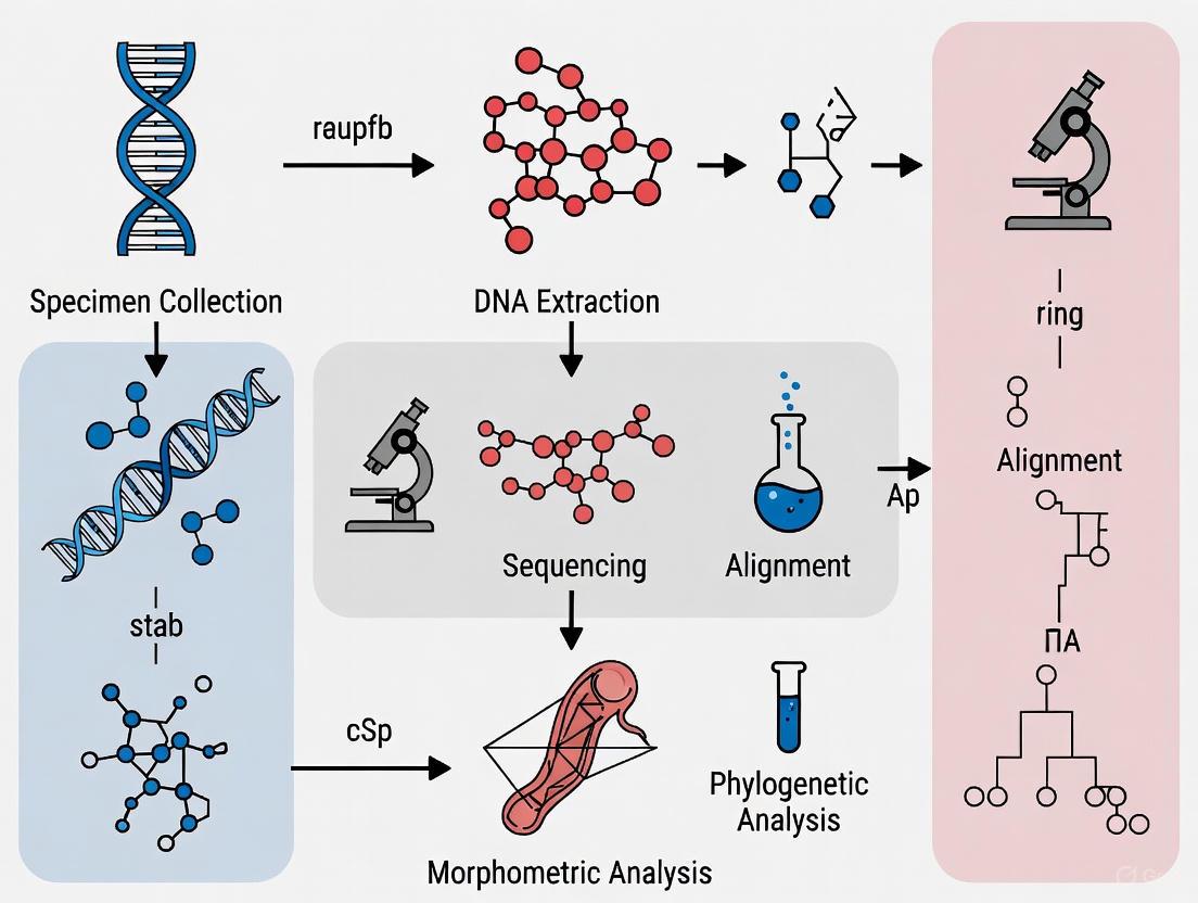
Integrated Workflow for Species Delimitation
The following diagram illustrates a comprehensive protocol for cryptic species discrimination integrating geometric morphometrics with complementary approaches:
Integrated Workflow for Cryptic Species Discrimination
Detailed Geometric Morphometrics Protocol
Based on established methodologies across multiple taxa [7] [6] [8], the following step-by-step protocol provides a standardized approach for cryptic species discrimination:
Phase 1: Sample Preparation and Image Acquisition
- Specimen Selection: Select adult specimens where possible to minimize ontogenetic variation. Ensure specimens represent the full geographical range of the putative species complex.
- Standardized Imaging: Capture high-resolution digital images using consistent orientation and scale. For 2D analysis, ensure the camera lens is perpendicular to the specimen plane. Use a solid-color background to facilitate subsequent image processing.
- Image Processing: Enhance images using software such as Adobe Photoshop or ImageJ by adjusting contrast and sharpness to improve landmark visibility. Crop images to focus on the anatomical structures of interest.
Phase 2: Landmark Digitation
- Landmark Selection: Identify homologous landmarks covering the entire structure of interest. Combine Type I (anatomical), Type II (mathematical), and Type III (constructed) landmarks as needed [7].
- Landmark Coordinate Collection: Use specialized software (e.g., tpsDig2) to record Cartesian coordinates (x, y) for each landmark across all specimens. For 3D data, collect (x, y, z) coordinates using appropriate digitization equipment.
- Quality Control: Check for landmark placement errors by visualizing all specimens simultaneously. Re-digitize outliers or specimens with evident placement inaccuracies.
Phase 3: Procrustes Superimposition and Data Preprocessing
- Generalized Procrustes Analysis (GPA): Perform GPA to remove the effects of size, position, and orientation through three sequential steps:
- Centering: Translate all configurations to a common origin (0,0)
- Scaling: Scale configurations to unit centroid size
- Rotation: Rotate configurations to minimize the sum of squared distances between corresponding landmarks
- Extraction of Shape Variables: The resulting Procrustes coordinates represent the shape variables for subsequent statistical analysis.
- Centroid Size Calculation: Compute centroid size (the square root of the sum of squared distances of all landmarks from their centroid) as a size variable for allometric analyses.
Phase 4: Statistical Analysis of Shape Variation
- Exploratory Analysis: Conduct Principal Component Analysis (PCA) on the covariance matrix of Procrustes coordinates to identify major patterns of shape variation and visualize specimen distribution in morphospace.
- Group Discrimination: Perform Discriminant Function Analysis (DFA) or Canonical Variate Analysis (CVA) to maximize separation between putative species groups and calculate classification accuracy.
- Hypothesis Testing: Use Procrustes ANOVA to test for significant shape differences between groups while accounting for allometric effects if necessary. Implement permutation tests (typically 10,000 iterations) to assess the statistical significance of Procrustes and Mahalanobis distances between groups [6].
- Allometry Analysis: Regress shape variables (Procrustes coordinates) against centroid size to quantify allometric patterns and test whether shape differences between groups are independent of size variation.
Phase 5: Visualization and Interpretation
- Thin-Plate Spline Visualization: Generate deformation grids to illustrate shape changes associated with principal components or discriminant functions.
- Mean Shape Comparison: Calculate and visualize consensus shapes for each putative species to identify regions of greatest morphological differentiation.
- Biological Interpretation: Relate statistical findings to biologically meaningful morphological differences, considering functional, ecological, or evolutionary implications.
Essential Research Reagents and Computational Tools
Successful implementation of geometric morphometrics protocols requires specific software tools and technical resources. The following table summarizes essential solutions for cryptic species research:
Table 3: Essential Research Reagents and Computational Tools for Geometric Morphometrics
| Tool Category | Specific Software/Package | Primary Function | Application Example |
|---|---|---|---|
| Landmark Digitization | tpsDig2 [7] [6] | Collection of landmark coordinates from digital images | Landmark placement on thrips head and thorax [6] |
| Data Management | tpsUtil [7] | Organization and management of landmark files | Creating tps files from multiple specimen images [7] |
| Shape Analysis | MorphoJ [7] [6] | Procrustes analysis, PCA, DFA, allometry analysis | Statistical comparison of head shape in Thrips species [6] |
| Comprehensive Analysis | R packages (geomorph, Momocs) [7] [6] | Advanced GM analysis and visualization | Procrustes ANOVA and permutation tests [6] |
| Image Processing | ImageJ [7] | Image enhancement and preprocessing | Background removal and contrast adjustment [7] |
| Molecular Validation | Geneious, MEGA | DNA sequence alignment and genetic distance calculation | COI barcoding of Barbirostris mosquito complex [4] |
Case Studies and Applications
Empirical Examples Across Taxa
The application of geometric morphometrics to cryptic species discrimination has yielded significant insights across diverse organisms:
Thrips (Insecta): Analysis of head and thorax shapes in Thrips species revealed significant morphological differences between quarantine-significant and non-significant species that were not detectable through traditional morphology [6]. Landmarks on the head and thoracic setae insertion points provided complementary discrimination power, with principal component analysis showing distinct clustering of species in morphospace.
Mosquitoes (Diptera): Wing geometric morphometrics of the Anopheles Barbirostris complex demonstrated moderate discrimination efficacy (74.29% accuracy based on wing shape) between three cryptic species (An. dissidens, An. saeungae, and An. wejchoochotei) that are important malaria vectors with distinct ecological roles [4].
Kissing Bugs (Hemiptera): Integration of head and pronotum shape analysis with ecological niche modeling improved delimitation of Triatoma pallidipennis haplogroups, revealing morphological differences concentrated in specific head regions that had taxonomic value for distinguishing genetically defined groups [8].
Marine Copepods (Crustacea): The Eurytemora affinis species complex, initially considered a classic example of cryptic species based on genetic evidence, was found to comprise pseudocryptic species after detailed morphological analysis using multivariate approaches and fluctuating asymmetry measurements [3].
Comparative Performance of Morphometric Methods
The relative performance of geometric morphometrics versus traditional linear morphometrics has been quantitatively evaluated in systematic studies:
Performance Comparison Between Morphometric Approaches
The discrimination of cryptic species represents a significant challenge in taxonomy, biodiversity assessment, and evolutionary biology. Traditional morphological methods often prove inadequate for this task due to their reliance on macroscopic characters, subjective character selection, and inability to quantify subtle shape variation. Geometric morphometrics provides a powerful alternative through its capacity for holistic shape characterization, explicit separation of size and shape variation, and robust statistical framework for group discrimination.
When integrated with molecular data and ecological niche modeling as part of an integrative taxonomic approach, geometric morphometrics significantly enhances our ability to detect and describe cryptic species diversity. This comprehensive approach is essential for accurate biodiversity assessment, understanding evolutionary processes, and informing conservation strategies where morphologically similar species may have distinct ecological requirements or disease vector capabilities.
Geometric morphometrics (GM) has emerged as a fundamental technique for the quantitative analysis of biological shape, providing robust tools for quantifying and visualizing morphology in evolutionary biology, taxonomy, and ecology. Unlike traditional morphometric approaches that rely on linear measurements, ratios, or angles, GM captures the complete geometric configuration of structures using Cartesian landmark coordinates [9]. This approach has proven particularly valuable in discriminating between cryptic species—lineages that are genetically distinct but superficially morphologically similar—where traditional taxonomic methods often fail [10] [11]. The power of GM lies in its ability to isolate shape variation from differences in size, position, and orientation through sophisticated statistical frameworks, enabling researchers to detect subtle morphological patterns that reflect underlying genetic and ecological differences [9] [10].
The analytical pipeline of GM transforms raw landmark coordinates into shape variables that can be analyzed using multivariate statistics, allowing researchers to test hypotheses about morphological variation, evolutionary relationships, and ecological adaptations. By preserving the geometric relationships among anatomical points throughout the analysis, GM facilitates visualization of shape changes along morphological gradients, providing intuitive interpretations of complex statistical results [12]. This protocol outlines the complete workflow from study design and data collection through statistical analysis and interpretation, with particular emphasis on applications in cryptic species discrimination research.
Fundamental Concepts and Data Types
Landmark Typology
Landmarks are discrete, homologous points that capture the geometry of biological structures. They are classified based on their anatomical and mathematical properties:
Table 1: Landmark Types in Geometric Morphometrics
| Landmark Type | Definition | Examples | Applications |
|---|---|---|---|
| Type I (Anatomical) | Points of clear biological significance at tissue junctions | Intersection of veins in insect wings, bone sutures | High reliability studies; skeletal morphology |
| Type II (Mathematical) | Points defined by geometric properties (maxima/minima of curvature) | Tip of a spine, deepest point of a notch | Capturing shape information where anatomical landmarks are sparse |
| Type III (Constructed) | Points defined by relative position to other landmarks | Midpoint between two landmarks, extremal points | Outlining complex shapes; supplementing Type I and II landmarks |
| Semilandmarks | Points along curves and surfaces that slide to minimize bending energy | Outline of a fish body, wing margins | Capturing smooth curves and surfaces without discrete landmarks |
Shape and Shape Space
In geometric morphometrics, "shape" is formally defined as all the geometric information that remains when differences in location, scale, and rotation are removed from an object [13]. The concept of "shape space" refers to the multidimensional space where each dimension corresponds to a shape variable, and each specimen is represented as a single point in this space [9]. The transformation of raw landmark coordinates into shape space occurs through Generalized Procrustes Analysis (GPA), which standardizes configurations by:
- Centering: Translating all configurations to a common origin (usually the centroid)
- Scaling: Scaling all configurations to unit centroid size
- Rotating: Rotating configurations to minimize the sum of squared distances between corresponding landmarks
This process results in Procrustes shape coordinates that occupy a curved manifold known as Kendall's shape space, which is typically approximated by a tangent space for subsequent statistical analysis using standard multivariate methods [14].
Quantitative Data in Geometric Morphometrics
Measurement Error Assessment
Comprehensive evaluation of measurement error is essential for ensuring the reliability of geometric morphometric data. Different sources of error contribute variably to the total variance in landmark configurations:
Table 2: Sources and Impacts of Measurement Error in Geometric Morphometrics
| Error Source | Error Type | Contribution to Total Variance | Impact on Statistical Classification |
|---|---|---|---|
| Imaging Device | Instrumental | Variable, depending on equipment | Moderate; affects all subsequent analyses |
| Specimen Presentation | Methodological | Can be substantial in 2D analyses | High; significantly affects group membership predictions |
| Interobserver Variation | Personal | Often substantial (>30% in some studies) | High; different digitizers yield different results |
| Intraobserver Variation | Personal | Variable based on experience and landmark clarity | Moderate; affects replicability of individual studies |
Research on vole molars has demonstrated that no two landmark dataset replicates exhibit identical predicted group memberships for recent or fossil specimens, emphasizing the critical need for standardization throughout data collection [12].
Classification Accuracy in Species Discrimination
Geometric morphometrics has demonstrated variable efficacy in discriminating between closely related species across different taxonomic groups:
Table 3: Classification Accuracy of Geometric Morphometrics in Species Discrimination
| Study Organism | Morphological Structure | Analytical Method | Classification Accuracy |
|---|---|---|---|
| Tabanus spp. (horse flies) | First submarginal wing cell | Outline-based GM | 86.67% |
| Tabanus spp. (horse flies) | Discal and second submarginal wing cells | Outline-based GM | 64.67%-68.67% |
| Thrips genus (8 species) | Head landmarks | Landmark-based GM with PCA | Statistically significant separation |
| Triatoma pallidipennis haplogroups | Head landmarks | Landmark-based GM | Significant differences in mean head shape |
| Triatoma pallidipennis haplogroups | Pronotum landmarks | Landmark-based GM | Limited discriminatory power |
Experimental Protocols
Complete Workflow for Landmark-Based Geometric Morphometrics
The following protocol provides a standardized approach for geometric morphometric analysis, with particular attention to applications in cryptic species discrimination:
Phase 1: Study Design and Image Acquisition
- Define Research Objectives: Clearly formulate hypotheses regarding morphological differentiation between putative cryptic species or populations.
- Determine Sample Size: Ensure sample size is approximately three times the number of landmarks to maintain statistical power [9].
- Standardize Imaging Protocol:
- Use consistent imaging equipment (camera, lens, lighting) throughout the study [12]
- Position specimens in consistent orientations to minimize presentation error
- For 2D analyses, ensure the camera lens is perpendicular to the specimen plane [15]
- Use adequate resolution (typically 2-10 MB file size) to clearly visualize landmark locations [15]
- Include Scale References: Incorporate scale bars in all images for size calibration when necessary.
Phase 2: Landmark Digitization
- Landmark Selection: Identify homologous anatomical points that adequately capture the shape of the structure:
- Landmark Ordering: Digitize landmarks in consistent order across all specimens [9].
- Error Reduction:
- For multiple observers, conduct training sessions to standardize landmark placement
- Consider having a single experienced observer digitize all specimens when possible [12]
- Re-digitize a subset of specimens to quantify intraobserver error
Phase 3: Data Preprocessing
- File Format Management: Use TPS series software (tpsUtil, tpsDig2) to manage and organize landmark data [15].
- Generalized Procrustes Analysis (GPA):
- Perform GPA to remove effects of size, position, and orientation
- Center configurations to their centroids
- Scale to unit centroid size
- Rotate to minimize Procrustes distances among corresponding landmarks
- Semilandmark Processing: Slide semilandmarks along tangent lines or planes to minimize bending energy [9].
Phase 4: Statistical Analysis
- Principal Component Analysis (PCA):
- Group Differentiation Tests:
- Classification Analysis:
- Implement discriminant function analysis (DFA) or canonical variate analysis (CVA) to assess classification accuracy
- Perform cross-validation to test the robustness of classification [10]
Phase 5: Visualization and Interpretation
- Shape Visualization: Use thin-plate spline (TPS) deformation grids to visualize shape differences between groups [9].
- Biological Interpretation: Relate statistical results to biological hypotheses about species boundaries, ecological adaptations, or evolutionary relationships [10].
Workflow Visualization
The Scientist's Toolkit: Essential Research Reagents and Software
Table 4: Essential Software Tools for Geometric Morphometric Analysis
| Software Tool | Primary Function | Application in Protocol | Availability |
|---|---|---|---|
| TPS Dig2 | Landmark digitization | Collecting 2D landmark coordinates from images | Free download |
| tpsUtil | TPS file management | Organizing and managing landmark files | Free download |
| MorphoJ | Statistical shape analysis | GPA, PCA, regression, group comparisons | Free download |
| R packages (geomorph, Momocs) | Comprehensive morphometric analysis | All analytical steps including advanced statistics | Open source |
| ImageJ | Image processing and analysis | Image preprocessing and measurement | Free download |
Table 5: Analytical Methods for Different Research Questions
| Research Question | Recommended Analysis | Example Application | Considerations |
|---|---|---|---|
| Overall shape variation | Principal Component Analysis (PCA) | Initial exploration of morphological space [14] [11] | Visualize extremes along PC axes |
| Group differences | Procrustes ANOVA, MANOVA | Testing differences between putative species [11] | Follow with pairwise comparisons |
| Classification accuracy | Discriminant Function Analysis (DFA) | Validating species boundaries [10] | Use cross-validation to avoid overfitting |
| Symmetry and asymmetry | Symmetry analysis [14] | Quantifying developmental instability | Partition symmetric/asymmetric components |
| Allometry | Multivariate regression | Shape vs. size relationships | Use centroid size as size variable |
Applications in Cryptic Species Discrimination
Geometric morphometrics has proven particularly valuable in discriminating cryptic species where traditional morphological characters are insufficient. In Triatoma pallidipennis, a Chagas disease vector, geometric morphometrics of head structures revealed significant shape differences among genetically distinct haplogroups that were morphologically indistinguishable using traditional taxonomic approaches [10]. Similarly, analyses of thrips head and thorax morphology demonstrated statistically significant differences among closely related species, providing a complementary approach to molecular methods for species identification [11].
The power of geometric morphometrics in cryptic species research stems from its ability to integrate multiple subtle morphological features into a comprehensive shape assessment. Rather than relying on discrete characters, the approach utilizes the continuous shape variation that reflects underlying genetic differences, often revealing morphological distinctions that align with molecular phylogenetic data [10]. When combined with ecological niche modeling, as demonstrated in the Triatoma study, geometric morphometrics provides a robust framework for delimiting species boundaries and understanding the ecological and evolutionary processes driving diversification [10].
For difficult taxonomic groups, outline-based methods applied to structures like wing cells can provide discriminatory power when landmark-based approaches are insufficient. In Tabanus species, the contour of the first submarginal wing cell achieved 86.67% classification accuracy, demonstrating the value of alternative approaches for challenging taxonomic problems [16]. This flexibility makes geometric morphometrics particularly suitable for cryptic species complexes where no single morphological character reliably distinguishes taxa.
Geometric morphometrics (GM) is a powerful statistical framework for quantifying biological shape, relying on coordinate-based data from anatomical landmarks. A cornerstone of modern GM is Procrustes analysis, a methodology used to superimpose landmark configurations by removing non-shape variations related to size, position, and rotation [17]. This process allows researchers to isolate and analyze pure shape differences, which is particularly crucial for discriminating between cryptic species—organisms that are nearly identical in appearance but belong to distinct taxonomic groups [18]. The name "Procrustes" originates from Greek mythology, referring to a bandit who forced his victims to fit his bed by stretching or cutting them off, analogous to how this analysis "forces" configurations into a common coordinate system [17].
In cryptic species research, where morphological differences are often subtle and localized, Procrustes-based GM provides the sensitivity required to detect and quantify these minor variations. By standardizing landmark configurations, it enables rigorous statistical comparisons of shape across individuals and populations. This protocol outlines the core principles, computational steps, and practical applications of the Procrustes protocol, with a specific focus on its role in discriminating morphologically similar species.
Theoretical Foundations
The Mathematical Basis of Shape Standardization
In Procrustes analysis, the shape of an object is formally defined as all the geometric information that remains after filtering out effects of translation, rotation, and scale [17]. This conceptualization treats shape as a member of an equivalence class, making Procrustes analysis a pure form of statistical shape analysis [17].
The mathematical procedure operates on configurations of landmark points. Consider an object represented by (k) points in (n) dimensions (typically 2D or 3D space). The configuration can be represented as a matrix: [ X = \begin{pmatrix} x1 & y1 & z1 \ x2 & y2 & z2 \ \vdots & \vdots & \vdots \ xk & yk & z_k \end{pmatrix} ] The Procrustes protocol standardizes such configurations through a sequence of operations performed iteratively in Generalized Procrustes Analysis (GPA) to optimally superimpose multiple specimens [17] [19].
Core Components of the Procrustes Superimposition
- Translation: Each configuration is translated so that its centroid (mean of all points) coincides with the origin of the coordinate system. This is achieved by subtracting the mean coordinate values from all points [17].
- Scaling: Configurations are scaled to a common size, typically unit centroid size, which is calculated as the square root of the sum of squared distances from each landmark to the centroid [17].
- Rotation: Configurations are rotated around the origin to minimize the Procrustes distance—the sum of squared distances between corresponding landmarks—between each specimen and a reference configuration [17].
Table 1: Mathematical Operations in Procrustes Analysis
| Operation | Mathematical Implementation | Effect on Shape Data |
|---|---|---|
| Translation | (X{\text{translated}} = X - 1\cdot mX^T) where (m_X) is the centroid [19] | Removes positional effects |
| Scaling | (X_{\text{scaled}} = X / \text{CS}) where CS is centroid size [17] | Removes size differences |
| Rotation | (X_{\text{rotated}} = X\cdot R) where R is the optimal rotation matrix [17] | Aligns configurations to minimize landmark deviations |
Computational Protocol
Generalized Procrustes Analysis (GPA) Algorithm
The standard approach for analyzing multiple specimens is Generalized Procrustes Analysis, which iteratively transforms all configurations toward a consensus. The following workflow details this computational protocol:
Diagram 1: Generalized Procrustes Analysis Iterative Workflow
The algorithm proceeds as follows:
- Initialization: Arbitrarily select one specimen as the initial reference configuration [17].
- Superimposition: For each configuration in the dataset:
- Consensus Update: Compute the mean shape from all superimposed configurations.
- Convergence Check: If the Procrustes distance between the new and previous mean shape exceeds a threshold, set the new mean as reference and return to step 2 [17].
Implementation in Statistical Software
Multiple R packages implement Procrustes analysis, each with specific capabilities:
geomorph::gpagen(): Performs GPA with options for sliding semi-landmarks [20]Morpho::procSym(): Performs Procrustes superimposition and symmetry analysis [20]shapes::procGPA(): Conducts basic Procrustes analysis [20]
For studies involving semi-landmarks (points along curves and surfaces), the gpagen() function can slide them according to bending energy criteria, which maintains biological realism while optimizing their positions [20].
Practical Applications in Cryptic Species Research
Case Study: Discriminating Lasiurus Bat Species
A recent application in chiropteran research demonstrates the power of Procrustes-based GM for cryptic species discrimination. Researchers analyzed skull morphology of Lasiurus borealis and Lasiurus seminolus—two morphologically similar bat species—using landmark data from multiple cranial views [18].
Table 2: Experimental Design for Bat Cryptic Species Discrimination
| Research Component | Implementation in Bat Study | Outcome |
|---|---|---|
| Sample | 72 L. borealis, 22 L. seminolus specimens | Adequate statistical power for discrimination |
| Landmarks | 14 fixed landmarks + 15 semi-landmarks (lateral cranium); 19 fixed landmarks + 6 semi-landmarks (ventral cranium) | Comprehensive shape characterization |
| Data Collection | Digital photographs with standardized angle; single observer to minimize error | Reduced measurement bias |
| Analysis | GPA followed by principal component analysis (PCA) | Successful species discrimination in all views |
The study found that despite their morphological similarity, the two species showed statistically significant differences in skull shape across all examined views (lateral cranium, ventral cranium, and lateral mandible) [18]. This demonstrates the sensitivity of Procrustes-based methods in detecting subtle but consistent morphological differences that traditional measurements might miss.
Impact of Methodological Choices
Several methodological considerations directly influence the effectiveness of Procrustes analysis for cryptic species discrimination:
- Sample Size: Reduced sample sizes increase shape variance and decrease precision of mean shape estimation [18]. Studies with insufficient samples may fail to detect subtle interspecific differences.
- Landmark Type and Density: Combinations of fixed landmarks and semi-landmarks provide optimal shape coverage. Over-sampling increases data collection time and reduces statistical power, while under-sampling misses biologically relevant shape information [21].
- Observer Error: Inter-operator differences can account for up to 30% of sample variation in shape data, potentially obscuring biological signals [22]. Standardized training and single-observer designs minimize this bias.
Research Reagent Solutions
Table 3: Essential Tools for Procrustes-Based Geometric Morphometrics
| Tool Category | Specific Examples | Function in Research |
|---|---|---|
| Digitization Software | tpsDig2 [18], Viewbox 4 [21] | Capture landmark coordinates from 2D images or 3D scans |
| 3D Scanning Hardware | Structured-light scanners (e.g., Artec Eva) [21] | Create high-resolution 3D models of specimens |
| Analysis Packages | geomorph (R) [20], Morpho (R) [20], shapes (R) [23] | Perform GPA, statistical analysis, and visualization |
| Specialized Superimposition Tools | tpsSuper [23], GRF-ND [23] | Conduct specific types of Procrustes superimposition |
Critical Considerations and Limitations
Measurement Error and Data Quality
The accuracy of Procrustes analysis is highly dependent on landmark precision. Studies using MRI data have shown that inter-operator differences can account for up to 30% of sample variation in shape data—a bias substantial enough to dominate biological signals like sexual dimorphism [22]. This emphasizes the need for:
- Comprehensive training of personnel in landmark identification
- Assessment of measurement error through replicate digitizations
- Blinding procedures during data collection to minimize observer bias [22]
Special Cases and Methodological Adaptations
Certain research contexts require modifications to standard Procrustes protocols:
- Articulating Structures: For kinetic structures like fish skulls or snake skeletons, where elements move independently, local superimposition methods separately align components before concatenating coordinates [24]. This approach isolates shape variation within elements while sacrificing information about their relative positions.
- Missing Data: For incomplete specimens (common in archaeological samples), statistical imputation methods can estimate missing landmark coordinates, though their effectiveness decreases with higher proportions of missing data [21].
- 3D vs. 2D Data: While 3D landmark data captures morphology more comprehensively, 2D approaches remain valuable for their accessibility, particularly when working with museum specimens or large sample sizes [18].
The Procrustes protocol provides an essential methodological foundation for shape analysis in geometric morphometrics, particularly in challenging research domains like cryptic species discrimination. By standardizing landmark configurations through translation, scaling, and rotation, it enables researchers to detect and quantify subtle morphological patterns that would otherwise remain obscured by variation in size, position, and orientation. The successful application to bat cryptic species demonstrates its practical utility, while ongoing methodological developments continue to expand its applicability to complex biological structures. As geometric morphometrics evolves, the Procrustes protocol remains central to rigorous shape comparison across diverse research contexts.
Within the framework of geometric morphometric (GM) protocols for cryptic species discrimination, the selection of anatomical structures is paramount. Wings, heads, and shells represent ideal candidates due to their complex, quantifiable shapes that are often under strong genetic and ecological control. This document provides detailed application notes and experimental protocols for the GM analysis of these structures, facilitating standardized research in systematics and phylogenetics.
Table 1: Common Landmarking Schemes for Key Anatomical Structures
| Anatomical Structure | Type of Organism | Recommended Number of Landmarks | Type of Landmarks (LM) | Key References (Example) |
|---|---|---|---|---|
| Wings | Insects (e.g., Drosophila, mosquitoes) | 12-16 | Type II (anatomical junctions of veins) | [1] |
| Heads | Fish, Lizards, Mammals | 20-30 | Type I (juctions of bony sutures) & Type II | [2] |
| Shells | Mollusks (Bivalves, Gastropods) | 2D: 15-25; 3D: 50+ | Semi-landmarks (outlines) | [3] |
Table 2: Statistical Power in Cryptic Species Discrimination
| Structure | Typical Procrustes Variance Explained (%)* | Discriminatory Power (Cross-Validated %) | Software Suites |
|---|---|---|---|
| Wings | 70-85% | 85-95% | MorphoJ, tps series |
| Heads | 60-80% | 75-90% | MorphoJ, EVAN Toolbox |
| Shells | 50-70% | 70-85% | tpsRelw, R (geomorph) |
*Percentage of total shape variance explained by the first two principal components in a typical cryptic species dataset.
Experimental Protocols
Protocol 3.1: Wing Preparation and Imaging (Diptera)
Application: Discrimination of cryptic mosquito species (Anopheles gambiae complex).
- Dissection: Under a stereo microscope, carefully remove the right wing from the thorax using fine-tipped forceps.
- Mounting: Place the wing on a microscope slide with a drop of Euparal mounting medium. Gently lower a coverslip, avoiding bubbles.
- Imaging: Capture a digital image using a compound microscope with a mounted camera at 40x magnification. Ensure the wing is perfectly flat and in full focus. Include a scale bar.
- Landmarking: In
tpsDig2, place Type II landmarks at the junctions of major wing veins (e.g., R-R1, R2-R3, etc.). A standard scheme uses 12 landmarks.
Protocol 3.2: Head Capsule Preparation and 3D Data Acquisition (Coleoptera)
Application: Morphometric analysis of cryptic beetle species.
- Fixation: Dissect the head capsule and clean soft tissue using 10% KOH solution.
- Staining (Optional): Soak in Acid Fuchsin to enhance contrast for micro-CT scanning.
- Micro-CT Scanning: Mount the specimen on a stub and scan using a SkyScan 1272 scanner at a 5 µm resolution.
- Reconstruction & Landmarking: Reconstruct the 3D model using NRecon software. In
Landmark Editor(IDAV), place 25 Type I landmarks on conserved anatomical points (e.g., eye margins, antennal sockets, clypeal sutures).
Protocol 3.3: Shell Outline Data Capture (Gastropoda)
Application: Discrimination of morphologically similar snail species.
- Standardization: Orient all shells with the apex vertical and the aperture facing the observer.
- Imaging: Photograph shells against a neutral background with a standardized scale using a DSLR camera on a copy stand.
- Outline Digitization:
- In
tpsUtil, create a TPS file from the images. - Open the TPS file in
tpsDig2. Use the "Outline" tool to digitize a series of 100 equidistant semi-landmarks along the shell's periphery, starting and ending at the shell apex. - Use
tpsRelwto slide the semi-landmarks to minimize bending energy, removing the effect of arbitrary starting points.
- In
Visualized Workflows
GM Analysis Workflow
GM Data Analysis Pathway
The Scientist's Toolkit
Table 3: Essential Research Reagents and Materials
| Item | Function in GM Analysis | Example Product / Specification |
|---|---|---|
| Fine-Tipped Forceps | Precise dissection of delicate structures (wings, legs). | Dumont #5 Inox Forceps |
| Stereomicroscope | For dissection and initial specimen observation. | Leica S9E with 10x-40x zoom |
| Compound Microscope with Camera | High-resolution imaging of 2D structures (wings, scales). | Olympus BX53 with DP27 camera |
| Micro-CT Scanner | Non-destructive 3D internal and external morphology data capture. | Bruker Skyscan 1272 |
| Standardized Scale Bar | Critical for calibrating image measurements and scale. | Pyser SGI Microscale (1mm) |
| Mounting Medium (Euparal) | Permanent mounting of translucent specimens for imaging. | Sigma-Aldrich Euparal |
| Landmarking Software | Digitizing coordinate points from images. | tpsDig2, MorphoJ |
| Statistical Software with GM Packages | Performing Procrustes superimposition and multivariate stats. | R (geomorph package), MorphoJ |
The Role of Principal Component Analysis (PCA) in Visualizing Morphospace
In geometric morphometrics (GM), morphospace is a mathematical space defined by shape variables, where each point represents the shape of an organism or structure. The concept of a shape space, specifically Kendall shape space, is a fundamental principle in GM; it is a non-Euclidean manifold where the distance between points corresponds to the degree of shape difference, independent of size, position, and orientation [25]. Principal Component Analysis (PCA) serves as a primary tool for exploring and visualizing this complex shape space. PCA operates on Procrustes shape coordinates—the standard shape variables in GM obtained after superimposing landmark configurations to remove non-shape variation [25]. The analysis works by generating a new set of uncorrelated variables, the Principal Components (PCs), which are linear combinations of the original shape variables and are ordered so that the first few retain most of the variation present in the original data [25]. This process creates a lower-dimensional, Euclidean tangent space that provides a linear approximation to the curved shape space, enabling the use of standard multivariate statistics and intuitive visualization of shape distributions and patterns [25].
The application of PCA in morphospace analysis is particularly powerful in cryptic species discrimination. When morphological differences are subtle and not easily discernible by traditional observation, PCA can reveal underlying patterns of shape variation that may correspond to genetically distinct lineages. For instance, in a study on thrips of the genus Thrips, PCA of head and thorax shapes successfully visualized morphological divergence among species, highlighting its utility for distinguishing taxa that are challenging to identify using traditional taxonomy [6].
Workflow and Protocol for PCA in Morphospace Analysis
The following diagram illustrates the standard workflow for a geometric morphometric analysis utilizing PCA, from data collection to the final visualization and interpretation of the morphospace.
Stage 1: Data Acquisition and Landmarking
Objective: To capture the geometry of biological structures in the form of 2D or 3D landmark coordinates.
Protocol:
- Sample Collection: Select specimens representing the groups of interest (e.g., potential cryptic species, different populations). Ensure sample sizes are adequate for robust statistical analysis.
- Landmark Definition: Define a set of anatomically homologous landmarks—discrete, biologically corresponding points that can be reliably located across all specimens [25]. For thrips discrimination, studies have used landmarks on the head and the insertion points of setae on the thorax [6].
- Data Capture:
- 2D Data: Capture high-resolution images of consistently oriented specimens. Use software like TPS Dig2 to digitize the 2D coordinates of each landmark on every image [6] [26].
- 3D Data: For more complex 3D structures, use a 3D digitizer, laser scanner, or CT/MRI scanning to obtain 3D landmark coordinates.
Considerations:
- Landmark Type: Combine Type I (discrete anatomical loci), Type II (maxima of curvature), and Type III (extremal points) landmarks as needed.
- Semi-landmarks: For curves and outlines, use semi-landmarks to capture shape information, which are later slid to minimize bending energy or procrustes distance, effectively making them geometrically homologous [27].
Stage 2: Procrustes Superimposition
Objective: To remove the effects of translation, rotation, and scaling from the raw landmark data, isolating pure shape information for analysis.
Protocol:
- Center: Translate all landmark configurations so that their centroid (center point) is at the origin (0,0).
- Scale: Scale all configurations to a standard size, typically to unit Centroid Size. Centroid Size is the square root of the sum of squared distances of all landmarks from their centroid, providing a size measure uncorrelated with shape for small variations [25].
- Rotate: Rotate the landmark configurations around their centroid to minimize the overall sum of squared distances between corresponding landmarks—a process known as Generalized Procrustes Analysis (GPA).
Output: The resulting Procrustes shape coordinates are the data upon which PCA is performed [25].
Stage 3: Principal Component Analysis and Morphospace Visualization
Objective: To reduce the dimensionality of the Procrustes shape coordinates and visualize the major trends of shape variation in a morphospace.
Protocol:
- Perform PCA: Conduct a PCA on the variance-covariance matrix of the Procrustes coordinates. This is standard functionality in GM software like MorphoJ [6] and the R package
geomorph[6]. - Interpret Output:
- Eigenvalues: Represent the variance explained by each Principal Component (PC). The first PC captures the greatest variance in the dataset, the second PC the next greatest, and so on.
- PC Scores: The position of each specimen along a PC axis. These scores are used to plot specimens in the morphospace.
- Eigenvectors (Loadings): Describe how the original shape variables contribute to each PC.
- Create Morphospace Plot: Generate a scatter plot using the first few PCs (e.g., PC1 vs. PC2) as the axes. Each point represents a specimen, and points closer together in the plot have more similar shapes.
- Visualize Shape Changes: Use the loadings to visualize the shape transformation associated with movement along a PC axis. This is typically done using thin-plate spline (TPS) deformation grids [25], which warp a reference shape (usually the mean shape) to show the shape at extremes (e.g., -0.1 and +0.1) of a PC axis.
Case Study Application: Discriminating Thrips Species
A study on eight species of thrips (Thrips genus) provides a clear example of PCA's application in a cryptic species context [6]. Researchers used landmark-based GM on the head and thorax of adult females to explore morphological differences.
Quantitative Results of PCA: The table below summarizes the PCA output from the analysis of head shape in thrips [6].
Table 1: PCA Results for Head Shape in Thrips Species [6]
| Principal Component | Variance Explained | Cumulative Variance |
|---|---|---|
| PC1 | 33.07% | 33.07% |
| PC2 | 25.94% | 59.01% |
| PC3 | 14.02% | 73.03% |
Visualization and Interpretation: The PCA revealed that the first three PCs accounted for over 73% of the total head shape variation [6]. The resulting morphospace (PC1 vs. PC2) showed distinct clustering. T. australis and T. angusticeps were identified as the most morphologically distinct species, occupying the extremes of the morphospace, while other species like T. hawaiiensis and T. palmi showed overlap [6]. The associated shape visualizations described these variations in terms of landmark displacements; for instance, the distinct species were characterized by a flattened head shape with specific vector movements affecting head height and width [6]. This demonstrates PCA's ability to quantify and visualize subtle shape differences that are critical for discriminating closely related species.
The Scientist's Toolkit: Essential Reagents and Software
Table 2: Key Research Tools for Geometric Morphometrics
| Tool / Reagent | Type | Primary Function in GM Protocol |
|---|---|---|
| MorphoJ | Software | Comprehensive GM analysis; performs Procrustes superimposition, PCA, and other statistical tests [6]. |
| TPS Dig2 | Software | Digitizes landmarks from 2D image files [6]. |
R package geomorph |
Software | Powerful R-based platform for GM, offering Procrustes ANOVA, PCA, and other advanced analyses [6]. |
| High-Resolution Scanner | Hardware | Captures high-quality 2D images of specimens for landmark digitization (e.g., 300 dpi or higher) [26]. |
| Microscribe or 3D Scanner | Hardware | Captures 3D landmark coordinates directly from physical specimens. |
| Procrustes Shape Coordinates | Data | The standardized shape variables obtained after superimposition; the direct input for PCA [25]. |
| Thin-Plate Spline (TPS) | Method | Algorithm for visualizing shape changes as smooth deformations of a reference grid [25]. |
Critical Analysis and Advanced Considerations
Strengths and Limitations of PCA in Morphospace Analysis
Strengths:
- Dimensionality Reduction: PCA efficiently simplifies complex, high-dimensional shape data into a few interpretable components.
- Exploratory Power: It is an unsupervised method, ideal for exploring data without a priori group assumptions, revealing unexpected patterns or outliers.
- Visualization: The morphospace plot provides an intuitive summary of the primary patterns of shape variation and similarity among specimens.
Limitations and Cautions:
- Linear Assumption: PCA is a linear technique, while shape space is non-linear. This is mitigated by the fact that the tangent space is a good local approximation [25].
- Variance ≠ Biological Importance: PCs are ordered by mathematical variance, which may not always reflect biologically or taxonomically meaningful variation.
- No Group Separation Guarantee: PCA describes total variation, not necessarily variation between pre-defined groups. For direct group discrimination, techniques like Canonical Variate Analysis (CVA) are often more powerful [28] [27].
Integrating PCA with Other Morphometric Tools
For robust cryptic species discrimination, PCA should be part of a broader analytical toolkit. The following diagram illustrates how PCA fits into an integrated workflow with other key analyses.
- Canonical Variate Analysis (CVA): Used after PCA to maximize separation among pre-defined groups. CVA is the method of choice for classification and generating a morphospace optimized for discrimination [28] [27].
- Cross-Validation: Essential for testing the predictive power of the classification. A leave-one-out procedure is common to estimate misclassification rates without bias [27].
- Molecular Validation: In cryptic species research, GM findings should be validated with independent data. For example, geometric morphometrics of sheep and goat teeth was confirmed by ZooMS (Zooarchaeology by Mass Spectrometry) [29], and studies on fish have highlighted cases where genetic lineages showed no morphological divergence despite GM analysis [30].
Practical GM Protocols: From Data Collection to Species Identification
Geometric morphometrics (GM) has revolutionized the quantitative analysis of biological shape by preserving the geometry of morphological structures throughout statistical analysis. For researchers focused on cryptic species discrimination, where traditional morphological characters often fail, GM provides a powerful tool for uncovering subtle but statistically significant shape differences. The foundation of any GM study lies in the precise capture of homologous shape data through the strategic placement of landmarks and semi-landmarks. These digital points serve as the primary data for analyzing shape variation within and between species, enabling researchers to visualize and quantify morphological patterns that are often invisible to the naked eye. The strategic selection of these points is particularly critical in cryptic species research, where morphological differences may be minimal yet biologically meaningful. This protocol details the methodologies for implementing landmark and semi-landmark strategies specifically within the context of discriminating closely related species.
Theoretical Foundation: Landmarks and Semi-Landmarks
Anatomical Landmarks
Landmarks are discrete, homologous points that correspond between specimens in a biological sample. They are defined by specific anatomical features and must be biologically comparable across all specimens in a study [9]. In the context of cryptic species discrimination, such as in a study of Thrips species, landmarks on the head and thorax can reveal subtle shape differences that distinguish quarantine-significant from non-significant species [6].
Table 1: Types of Anatomical Landmarks and Their Applications in Cryptic Species Research
| Landmark Type | Definition | Example | Utility in Cryptic Species |
|---|---|---|---|
| Type I (Topological) | Defined by discrete juxtapositions of tissues (e.g., holes, sutures). | Setal insertion points on thrips mesonotum and metanotum [6]. | High homology; excellent for quantifying structural differences in sclerotized body parts. |
| Type II (Geometric) | Defined by a point of maximum curvature or a local extremum of a shape. | Tips of cephalic setae in thrips [6]. | Good for capturing overall shape outlines; may be more variable. |
| Type III (Extreme) | Defined as endpoints or extreme points of a structure. | Most posterior point of the head capsule in thrips [6]. | Useful for capturing overall size and gross shape; homology must be carefully considered. |
Semi-Landmarks
Semi-landmarks are used to capture the shape of morphological structures that lack discrete, homologous points along their contours, such as curves and surfaces [9]. They are essential for quantifying the shape of smooth outlines, which often contain valuable taxonomic information. The process involves defining a start and end point with traditional landmarks and then placing a series of points along the curve between them. These points are then "slid" during the Procrustes superimposition process to minimize the bending energy between specimens, thus allowing them to function as homologous points in the analysis [9]. In fish morphology studies, for example, the addition of semi-landmarks on curves has been shown to provide a clearer differentiation of species within the morphospace [31].
Experimental Protocols and Workflows
Workflow for a Geometric Morphometric Study
The following diagram illustrates the standardized workflow for a geometric morphometric study, from initial design to final interpretation, ensuring reliable and reproducible results.
GM Study Workflow
Protocol: Landmark Data Collection for Cryptic Insect Species
The following detailed protocol is adapted from a study on Thrips species, which successfully used GM to distinguish morphologically similar insects [6].
Step 1: Specimen Preparation and Imaging
- Select slide-mounted adult specimens to ensure standardization.
- Obtain high-resolution digital images using a standardized microscope and camera setup. Consistent lighting and magnification are critical.
- Process images using software like Adobe Photoshop to enhance contrast and sharpness, ensuring landmark locations are clearly visible [6].
Step 2: Landmark Digitization
- Use specialized software such as TPSDig2 [6] [32] to record the Cartesian (x, y) coordinates of each predefined landmark.
- For the head, landmarks may include points on the compound eyes, ocelli, and the anterior and posterior margins of the head capsule [6].
- For the thorax, landmarks can include setal insertion points on the mesonotum and metanotum [6].
- Digitize all specimens in a randomized order to avoid systematic bias.
Step 3: Data Standardization via Procrustes Superimposition
- Import coordinate data into an analysis program such as MorphoJ [6] [33] or the geomorph package in R [34].
- Perform a Generalized Procrustes Analysis (GPA). This procedure removes the effects of size, position, and orientation by:
- The resulting Procrustes shape coordinates are the data used for all subsequent statistical analyses.
Protocol: Handling Curves and Surfaces with Semi-Landmarks
This protocol is critical for analyzing structures that lack discrete landmarks, as demonstrated in studies of fish morphology [31] and human hand shape [32].
Step 1: Define the Curve
Step 2: Place Semi-Landmarks
- Place a series of points along the curve between the fixed landmarks. The number of semi-landmarks should be consistent across all specimens for a given curve.
- Software like TPSDig2 can facilitate the even placement of these points.
Step 3: Sliding Semi-Landmarks
- During the Procrustes superimposition process, the semi-landmarks are allowed to "slide" along tangents to the curve. This minimizes the artificial variance introduced by their initial placement and optimizes their correspondence across specimens based on the bending energy of the thin-plate spline [9].
- Programs like MorphoJ and geomorph can perform this sliding step automatically.
The Scientist's Toolkit
Table 2: Essential Research Reagents and Software for Geometric Morphometrics
| Tool Name | Type | Primary Function | Application in Cryptic Species |
|---|---|---|---|
| TPSDig2 | Software | Digitize landmarks and semi-landmarks from 2D images [6] [32]. | Precise coordinate data acquisition from insect, fish, or other specimen images. |
| MorphoJ | Software | Integrated GM analysis: Procrustes fit, PCA, CVA, regression [33]. | User-friendly platform for statistical shape analysis and group discrimination. |
| geomorph (R package) | Software | Advanced GM analyses in a statistical programming environment [34]. | Flexible, powerful analysis for complex designs; enables customization and scripting. |
| High-Resolution Microscope & Camera | Hardware | Capture detailed, standardized digital images of specimens. | Essential for imaging small structures in insects where landmarks are minute. |
| Slide-Mounted Specimens | Specimen Prep | Standardize specimen orientation and ensure 2D comparability. | Critical for reducing postural variance in small insect studies (e.g., thrips [6]). |
Data Analysis and Visualization Strategies
Core Analytical Techniques
After Procrustes superimposition, the shape variables are analyzed using multivariate statistics.
Principal Component Analysis (PCA): This is often the first step in exploring shape variation. PCA reduces the dimensionality of the shape data to a few Principal Components (PCs) that describe the major axes of shape variation within the entire sample. In the Thrips study, the first three PCs of head shape accounted for over 73% of the total variation, successfully separating species like T. australis and T. angusticeps in the morphospace [6].
Canonical Variate Analysis (CVA): This technique is paramount for cryptic species discrimination. CVA finds the axes that maximize the separation between pre-defined groups (e.g., species) while minimizing the variation within them. It is particularly useful for highlighting the specific shape features that best distinguish one species from another.
Procrustes ANOVA: Used to test for statistically significant differences in shape between groups. This analysis tests whether the Procrustes distances between group mean shapes are larger than would be expected by chance alone [6].
Visualizing Shape Changes
A key advantage of GM is the ability to visualize shape changes associated with statistical outputs.
Deformation Grids (Thin-Plate Splines): These grids visually warp from the consensus (mean) shape to the target shape (e.g., a species mean or an extreme along a PC axis). The grid deformation allows for an intuitive interpretation of which anatomical regions are expanding, contracting, or bending [9]. This is invaluable for understanding the biological meaning behind statistical differences.
Vector Plots: These diagrams show the direction and magnitude of landmark displacement between two shapes. In the Thrips study, vector plots revealed that head shape differences were driven by opposing vectorial movements of landmarks associated with head height and width [6].
Application Note: Case Study in Thrips Species Discrimination
A landmark study on eight species of thrips of quarantine significance demonstrates the power of this approach. Researchers applied 11 landmarks to the head and 10 to the thorax (setal bases). The analysis revealed statistically significant differences in both head and thoracic morphology. The PCA of head shape showed distinct clustering, with T. australis and T. angusticeps being the most morphologically distinct. Notably, when the landmark set for one body region (e.g., head) did not show clear separation, the other set (thorax) provided complementary discriminatory power, as was the case for T. nigropilosus, T. obscuratus, and T. hawaiiensis [6]. This case study underscores the importance of selecting multiple, functionally relevant landmark sets to maximize the chances of discriminating cryptic species.
Imaging and Digitization Best Practices for High-Quality Data
In the field of geometric morphometrics (GM) for cryptic species discrimination, the fidelity of digital representations of specimens is paramount. The accuracy of subsequent analyses, including landmark placement and shape differentiation, is entirely dependent on the quality of the initial imaging and digitization processes [6]. Proper digitization extends beyond simple scanning; it is a comprehensive approach encompassing careful planning, adherence to technical standards, robust quality control, and accurate metadata creation to ensure high-quality digital conversions suitable for scientific research [35]. This document outlines established best practices and protocols for creating high-quality digital assets specifically for geometric morphometric research on cryptic species, such as thrips and other challenging taxa.
Technical Standards for Scientific Imaging
Adherence to established technical standards during image acquisition ensures data integrity, enables reproducibility, and facilitates long-term preservation. The following specifications provide a foundation for high-quality scientific imaging.
Table 1: Technical Standards for High-Quality Scientific Imaging
| Parameter | Minimum Recommended Specification | Enhanced Specification | Application Context |
|---|---|---|---|
| Resolution | 600 DPI [35] | > 600 DPI (e.g., 1200 DPI for micro-features) | Standard specimen imaging; fine-detail capture (e.g., setae, micro-sculpturing) |
| Bit Depth | 8-bit grayscale / 24-bit color [35] | 48-bit color (16-bit per channel) | Maximizing color/tonal accuracy for subtle feature discrimination |
| File Format (Master) | TIFF (uncompressed) [35] [36] | TIFF (uncompressed) | Archival master files, long-term preservation |
| Color Management | sRGB color space | Adobe RGB or ProPhoto RGB | Ensuring consistent color reproduction across devices |
| Lighting | Consistent, diffuse illumination to minimize shadows | Cross-polarized lighting to eliminate glare | Standard imaging; imaging glossy or reflective specimens |
The Federal Agencies Digital Guidelines Initiative (FADGI) provides a widely recognized benchmark for digitization quality, with a 3-star rating indicating high-quality images suitable for long-term preservation [35]. For geometric morphometric studies, where subtle shape differences are critical, exceeding these minimums is often necessary. Research on thrips species, for instance, relies on high-resolution images of heads and thoraxes for precise landmark digitization [6].
Digitization Workflow Protocol
A standardized, multi-stage workflow is critical for managing digitization projects, ensuring consistency, and maintaining quality throughout the process. The following protocol outlines the key stages from preparation to final delivery.
Figure 1: Sequential workflow for high-quality specimen digitization, from preparation to archiving.
Stage 1: Specimen Preparation
Before image capture, specimens must be carefully prepared. This includes cleaning to remove debris and stabilizing the specimen to ensure a consistent, repeatable orientation. Fragile items may require special handling [36]. The imaging stage should include a scale bar and color calibration target within the frame to provide spatial and color reference, which is crucial for subsequent morphometric analyses [6].
Stage 2: Image Acquisition
This core stage involves capturing the digital image according to the predefined technical standards (Table 1). Equipment must be properly calibrated. For reproducible geometric morphometrics, consistent camera angle, lighting, and specimen orientation are non-negotiable. The use of a motorized stage on a microscope can facilitate the capture of multiple focal planes for focus stacking, ensuring entire structures are in sharp focus.
Stage 3: Quality Control (QC)
QC is an iterative process, not a single step. In large-scale projects, even a 0.1% error rate can translate to thousands of flawed images, compromising data integrity [36]. Each image must be reviewed for focus, contrast, completeness, and the absence of artifacts. In geometric morphometric studies, this includes ensuring that all landmarks are visible and not obscured. Automated tools can flag common issues, but manual review by a trained technician is essential for spotting subtle problems [35] [36].
Stage 4: File Processing and Delivery
The final stage involves processing the master archival file (e.g., TIFF) into derivative formats suitable for landmarking software. Metadata should be embedded into the image files. A robust backup strategy, including multiple copies in geographically separate locations, is essential for digital preservation [35].
Quality Control and Metadata Framework
Rigorous quality control and comprehensive metadata creation are foundational to producing reliable, discoverable, and reusable scientific image data.
Quality Control Benchmarks
Quality should be measured against objective benchmarks. The FADGI star rating system is an industry standard that evaluates resolution, tonal and color accuracy, and other factors [35]. For morphometrics, additional project-specific checks are needed, such as verifying the clarity of setal insertion points used as landmarks in thrips research [6]. Effective QC involves multiple checkpoints and a combination of automated and manual review to catch errors like skewed orientation, blurry images, or incorrect file naming [37].
Metadata Creation
Accurate and comprehensive metadata is crucial for the management, retrieval, and long-term usability of digitized specimens. Without it, even perfectly scanned images become difficult to find and use [35]. Metadata should be captured at the time of imaging.
Table 2: Essential Metadata Schema for Morphometric Specimen Images
| Category | Description | Example |
|---|---|---|
| Descriptive | Information about the specimen's identity and origin. | Genus: Thrips, Species: australis, Collection Location: California, USA |
| Administrative | Information about the image file and its creation. | File Format: TIFF, Creation Date: 2025-11-26, Resolution: 1200 DPI |
| Technical | Technical specifications of the imaging process. | Microscope Magnification: 50x, Camera Model: [Model], Lighting: Cross-Polarized |
| Structural | Describes relationships between files (e.g., multiple views of one specimen). | Is Part Of: Series T_aus_001, View: Dorsal |
| Rights | Information about usage and access permissions. | Copyright: Institution Name, License: CC-BY-NC |
Common metadata standards include Dublin Core (a minimum for resource description) and more complex schemas like MARC or MODS [35]. Capturing this information systematically at the file level is a best practice for data management.
Application to Geometric Morphometrics
The imaging and digitization protocols described above are directly applicable to geometric morphometric research, as demonstrated in studies of cryptic species.
Case Implementation: Thrips Species Discrimination
A 2025 study on quarantine-significant thrips of the genus Thrips exemplifies the application of these protocols [6]. Researchers used slide-mounted adult females with high-resolution images. The image processing protocol involved cropping images to the target tagma (head or thorax) and enhancing them through higher contrast and sharpening using software like Adobe Photoshop. Landmarks were then digitized on the head (11 landmarks) and thorax (10 landmarks around setae) using specialized software (TPS Dig2). The Cartesian coordinates from these landmarks were processed using a Procrustes fit analysis to remove the effects of size, position, and rotation, allowing for pure shape comparison [6].
Analysis Workflow
The digitization and landmarking process feeds directly into the core geometric morphometrics analysis workflow, which can be visualized as follows:
Figure 2: Core analytical workflow in geometric morphometrics, from image to statistical result.
This study successfully differentiated species based on head and thorax shape, highlighting the power of GM when applied to high-fidelity digital images. The results demonstrated that GM can identify taxa challenging to distinguish using traditional taxonomy alone, proving particularly valuable for morphologically conservative groups [6].
The Scientist's Toolkit: Research Reagent Solutions
A successful digitization pipeline requires both specialized hardware and software. The following table details essential tools for a morphometrics-focused imaging lab.
Table 3: Essential Research Reagents and Tools for a Morphometrics Imaging Lab
| Tool Category | Specific Examples & Functions |
|---|---|
| Image Capture | Motorized Microscope & Camera System: Enables automated capture of multiple focal planes. Specimen Holder & Micro-positioning Stage: Ensures consistent, repeatable specimen orientation for valid comparisons. Cross-Polarized Lighting Fixtures: Eliminates glare and specular highlights from reflective specimen surfaces. |
| Calibration | Standardized Scale Bar (Stage Micrometer): Provides spatial reference in images for accurate measurement. Color Calibration Target (e.g., X-Rite ColorChecker): Ensures faithful color reproduction across imaging sessions. |
| Software | Image Editing (e.g., Adobe Photoshop): For cropping, minor contrast enhancement, and file format conversion [6]. Landmark Digitization (e.g., TPS Dig2): Specialized software for precise placement of landmarks on digital images [6]. Morphometric Analysis (e.g., MorphoJ, R geomorph package): For Procrustes superimposition, Principal Component Analysis (PCA), and statistical testing of shape differences [6]. |
| Data Management | Digital Asset Management (DAM) System: For storing, backing up, and embedding metadata into master image files. Laboratory Information Management System (LIMS): Tracks specimen provenance and links physical specimens to their digital assets and metadata. |
The Anopheles barbirostris complex comprises at least six formally recognized species that are morphologically indistinguishable yet play vastly different roles in disease transmission [38]. In Thailand, key members include An. barbirostris sensu stricto (s.s.), An. dissidens, An. saeungae, and An. wejchoochotei [38] [39]. The inability to accurately identify these species using traditional morphological keys has significantly hampered studies of their bionomics and vector competence [38] [40]. While molecular techniques such as multiplex PCR and DNA barcoding provide definitive identification, they are often resource-intensive, requiring specialized equipment and reagents [41]. Geometric morphometrics (GM) offers a complementary, cost-effective tool for discriminating among these cryptic species by analyzing the quantitative shape and size of mosquito wings [41] [42].
The following diagram illustrates the integrated workflow for identifying species within the Anopheles barbirostris complex, combining wing geometric morphometrics with molecular validation.
Comparative Performance of Identification Techniques
The table below summarizes the performance characteristics of different species identification methods as applied to the Anopheles barbirostris complex.
Table 1: Performance Comparison of Identification Techniques for the Anopheles barbirostris Complex
| Method | Key Principle | Reported Accuracy/Performance | Major Advantages | Major Limitations |
|---|---|---|---|---|
| Wing Geometric Morphometrics | Analysis of wing venation patterns using landmark coordinates [41]. | 74.29% (cross-validated reclassification based on wing shape) [41] [42]. | Cost-effective; rapid once reference library is established; preserves specimen for other analyses [41]. | Lower accuracy than molecular methods; requires specialized software and training; effectiveness varies by complex [41] [43]. |
| DNA Barcoding (COI gene) | Analysis of sequence variation in a standardized gene region (~658 bp of COI) [41]. | Clear species groups in phylogenies; low intraspecific (0.27-0.63%) vs. high interspecific (1.92-3.68%) distances [41]. | High reliability and resolution; creates a reusable digital database (BOLD) [41]. | Higher cost and technical requirements; cannot identify damaged specimens; potential lack of barcoding gap in some complexes [43]. |
| Multiplex PCR (ITS2/COI) | Amplification of species-specific DNA fragments using tailored primers in a single reaction [38] [39]. | 100% agreement with sequencing for validated species; successfully identified 5 species in Thailand [38] [39]. | High-throughput; unambiguous results; considered a gold standard [38]. | Requires prior knowledge of species for primer design; cannot detect new, unknown species [39]. |
| Morphological Identification | Microscopic examination of external characteristics using taxonomic keys [44]. | Highly variable (0-92.1%); most accurate for primary, expected species [44]. | Low immediate cost; widely applicable in the field. | Unreliable for cryptic species; requires high expertise; susceptible to damage and phenotypic plasticity [38] [44]. |
Detailed Wing Geometric Morphometrics Protocol
Specimen Preparation and Imaging
- Specimen Source: Collect adult female mosquitoes using methods such as human landing catches (HLC) or CDC light traps [41]. Store specimens in a way that minimizes damage to the wings.
- Wing Removal: Under a stereomicroscope, carefully detach the right wing from the thorax using fine-forceps.
- Mounting: Place the wing on a microscope slide with the dorsal side facing up, using a small drop of distilled water or mounting medium to secure it flat under a coverslip.
- Image Acquisition: Capture a digital image of the wing using a microscope equipped with a camera. Ensure the magnification is consistent across all samples, and include a scale bar for calibration.
Landmark Digitization
- Landmark Scheme: Digitize 12 Type II landmarks located at the junctions of wing veins. These landmarks are biologically homologous across all specimens [41].
- Software: Use specialized morphometrics software such as tpsDig2 (available from the SUNY Stony Brook Morphometrics website) to place the landmarks on the digital image.
- Precision: Perform all digitization by the same trained individual to minimize observer bias. For assessing measurement error, a subset of wings should be digitized at least twice on separate days.
Table 2: Wing Venation Landmark Definitions for the Anopheles barbirostris Complex
| Landmark Number | Anatomic Location on Wing |
|---|---|
| 1 | Junction of the humeral vein and the costal margin |
| 2 | Junction of the costal vein and the subcostal vein |
| 3 | Distal end of the radial sector (Rs) vein |
| 4 | Junction of the radial vein (R4+5) and the cross-vein r-m |
| 5 | Junction of the medial vein (M1+2) and the cross-vein r-m |
| 6 | Junction of the medial vein (M3+4) and the cross-vein m-cu |
| 7 | Junction of the cubital vein (CuA) and the cross-vein m-cu |
| 8 | Junction of the anal vein (CuP) and the posterior margin |
| 9 | Junction of the medial vein (M1+2) and the cross-vein m-m |
| 10 | Junction of the medial vein (M3+4) and the medial cell |
| 11 | Junction of the cubital vein (CuA) and the cubital cell |
| 12 | Junction of the anal vein (CuP) and the anal cell |
Data Analysis
- Generalized Procrustes Analysis (GPA): This statistical procedure removes the effects of size, position, and rotation from the landmark coordinates, leaving only the variation in shape for analysis.
- Statistical Classification:
- Use Discriminant Analysis (DA) or Canonical Variate Analysis (CVA) to find the combination of shape variables that best separates the pre-defined species groups (whose identity is confirmed by molecular methods).
- Perform a cross-validation test (e.g., Leave-One-Out) to calculate the unbiased reclassification accuracy of the model [41].
- Visualization: Generate a CVA scatterplot to visualize the separation between species groups based on their wing shapes.
The Scientist's Toolkit: Research Reagent Solutions
Table 3: Essential Materials and Reagents for Identification of the Anopheles barbirostris Complex
| Item | Function/Application | Specific Example / Note |
|---|---|---|
| DNA Extraction Kit | Isolation of genomic DNA from mosquito legs or wings for molecular validation. | Pure Link Genomic DNA Mini Kit [39] or DNeasy Blood & Tissue Kit [40]. |
| PCR Reagents | Enzymes and nucleotides for DNA amplification in multiplex PCR or barcoding. | GoTaq G2 Flexi DNA Polymerase, MgCl₂, dNTPs, reaction buffer [38]. |
| Species-Specific Primers | Amplification of diagnostic DNA fragments for member species of the complex. | COI-based multiplex primers for An. barbirostris s.s., An. dissidens, An. saeungae, An. wejchoochotei, and An. barbirostris A3 [39]. |
| Agarose Gel Electrophoresis System | Visualization and confirmation of PCR products based on their size. | Standard 2% agarose gel stained with GelRed or Midori Green DNA stain [38] [43]. |
| Geometric Morphometrics Software | Digitization of wing landmarks and statistical shape analysis. | tpsDig2 (digitization), MorphoJ or R (GPA and DA/CVA) [41]. |
| Silica Gel | Preservation of field-collected mosquito specimens for DNA and morphological integrity. | Store individual specimens in 1.5 ml tubes with silica gel [38] [40]. |
Wing geometric morphometrics presents a valuable and accessible tool for the preliminary identification or population-level screening of cryptic species within the Anopheles barbirostris complex, achieving a moderate classification accuracy of 74.29% [41] [42]. Its utility is maximized when integrated into a framework that uses molecular techniques for initial reference library building and ongoing validation. This integrated approach, leveraging the strengths of both morphology and molecular biology, is crucial for clarifying the distribution, bionomics, and vector status of each species, thereby informing targeted and effective malaria control strategies.
Application Notes
Accurate identification of thrips species is critical for plant biosecurity and preventing the introduction of quarantine-significant pests. The genus Thrips contains over 280 species worldwide, many of which are agricultural pests and virus vectors [6]. Traditional morphological identification is challenging due to small size and minimal distinguishing characteristics, particularly in morphologically conservative taxa and species complexes [6]. Geometric morphometrics (GM) provides a powerful complementary approach by quantifying subtle shape variations that are difficult to discern visually.
This case study demonstrates the application of landmark-based GM to discriminate between quarantine-significant and common thrips species using head and thoracic structures. The protocol offers taxonomists and regulatory scientists a standardized method for rapid identification of frequently intercepted species at ports of entry [6].
Key Findings and Quantitative Data
Analysis of eight Thrips species (four quarantine-significant, four common) revealed statistically significant differences in head and thorax morphology. Principal Component Analysis (PCA) of head shape variation showed the first three principal components accounted for 73.03% of total variance (PC1=33.07%, PC2=25.94%, PC3=14.02%) [6]. Species exhibited distinct clustering within the morphospace, with T. australis and T. angusticeps identified as the most morphologically distinct in head shape [6].
Table 1: Procrustes and Mahalanobis Distances for Head Shape Between Selected Thrips Species
| Species Comparison | Procrustes Distance | Mahalanobis Distance | p-value |
|---|---|---|---|
| T. angusticeps vs T. australis | 0.0921 | 7.7693 | <0.0001 |
| T. angusticeps vs T. hawaiiensis | 0.0564 | 4.6475 | <0.0001 |
| T. angusticeps vs T. palmi | 0.0587 | 5.2732 | <0.0001 |
| T. australis vs T. hawaiiensis | 0.0506 | 4.0295 | <0.0001 |
| T. australis vs T. palmi | 0.0533 | 4.2026 | <0.0001 |
| T. hawaiiensis vs T. palmi | 0.0244 | 2.3438 | 0.0014 |
Thorax shape analysis provided complementary discriminatory power, with T. nigropilosus, T. obscuratus, and T. hawaiiensis showing the greatest divergence in thoracic morphology [6]. The findings demonstrate GM's efficacy for discriminating cryptic species within this genetically complex genus.
Experimental Protocols
Protocol 1: Specimen Preparation and Imaging
Purpose: Standardized preparation of thrips specimens for geometric morphometric analysis.
Materials:
- Slide-mounted adult female thrips specimens
- High-resolution microscope with camera system
- Image editing software (e.g., Adobe Photoshop)
- USDA-APHIS-PPQ ImageID database (or equivalent)
Procedure:
- Specimen Selection: Select confirmed adult female specimens previously identified by taxonomic specialists [6].
- Slide Mounting: Ensure specimens are properly slide-mounted using standard entomological techniques.
- Image Acquisition: Capture high-resolution digital images using standardized microscopy protocols.
- Image Enhancement: Process images using Photoshop or equivalent software:
- Crop images to isolate target tagma (head or thorax)
- Enhance contrast and sharpness for landmark clarity [6]
- Quality Control: Verify image quality and consistency across all specimens.
Protocol 2: Landmark Digitization
Purpose: Capture homologous anatomical points for shape analysis.
Materials:
- TPS Dig2 software (v2.17 or newer)
- Processed head and thorax images
Landmark Configuration:
- Head Landmarks: Digitize 11 Type II landmarks representing biologically homologous points [6]:
- Anterior and posterior points of compound eyes
- Ocellar setae insertion points
- Head capsule vertices
- Thorax Landmarks: Digitize 10 setal insertion points on mesonotum and metanotum [6]
Procedure:
- Software Setup: Initialize TPS Dig2 and import image files.
- Landmark Placement: Systematically digitize all landmarks for each specimen.
- Data Export: Save Cartesian coordinates for statistical analysis.
Protocol 3: Statistical Shape Analysis
Purpose: Analyze shape variation and test for significant differences between species.
Materials:
- MorphoJ software (v1.07a or newer)
- R statistical environment with geomorph and ggplot2 packages
- Landmark coordinate data
Procedure:
- Procrustes Superimposition:
- Import landmark coordinates into MorphoJ
- Perform Generalized Procrustes Analysis to remove effects of size, position, and rotation [6]
- Generate Procrustes coordinates for statistical analysis
Principal Component Analysis (PCA):
- Compute covariance matrix of Procrustes coordinates
- Perform PCA to visualize morphospace distribution [6]
- Interpret principal components relative to percentage of variance explained
Statistical Testing:
Visualization:
- Generate deformation grids and wireframes to illustrate shape changes
- Create morphospace plots showing species distribution [6]
Diagram 1: Geometric Morphometrics Workflow for Thrips Identification
The Scientist's Toolkit: Research Reagent Solutions
Table 2: Essential Materials and Software for Thrips Geometric Morphometrics
| Item Category | Specific Product/Software | Function in Protocol |
|---|---|---|
| Imaging Software | Adobe Photoshop v26.0+ | Image enhancement, contrast adjustment, and cropping [6] |
| Landmark Digitization | TPS Dig2 v2.17 | Precise placement of anatomical landmarks on digital images [6] |
| Shape Analysis | MorphoJ v1.07a | Procrustes superimposition, PCA, and statistical shape analysis [6] |
| Statistical Computing | R Environment with geomorph & ggplot2 packages | Advanced statistical testing and visualization [6] |
| Reference Database | USDA-APHIS-PPQ ImageID | Verified specimen identification and reference images [6] |
| Microscopy | High-resolution compound microscope with camera | Detailed imaging of minute morphological structures [6] |
Troubleshooting and Technical Notes
Measurement Error: Conduct preliminary tests to estimate measurement error by repeating landmark digitization [26]. In leaf morphology studies, measurement error has been shown to be negligible with proper protocol standardization [26].
Landmark Homology: Ensure consistent placement of Type II landmarks across all specimens. Practice landmark identification on training specimens before formal data collection.
Sample Size: Aim for balanced design with equal numbers per species when possible to facilitate computation and avoid weighting bias [26].
Complementary Analysis: Use both head and thorax landmarks as they may provide complementary discriminatory power when one set alone shows insufficient variation [6].
This protocol provides a robust framework for applying geometric morphometrics to thrips identification, particularly valuable for discriminating cryptic species of quarantine significance in regulatory environments.
Accurate species discrimination is a fundamental challenge in deep-sea biodiversity research, particularly for taxa exhibiting cryptic diversity where significant genetic divergence is accompanied by minimal morphological variation [45]. The isopod family Macrostylidae represents a quintessential example of this problem; these organisms display a global distribution from sublittoral to hadal zones but exhibit remarkably low morphological disparity despite high molecular divergence [45]. This case study details the application of geometric morphometric (GM) techniques to analyze pleotelson shape variation in macrostylid isopods, establishing a standardized protocol for cryptic species discrimination within broader taxonomic research.
Geometric morphometrics has emerged as a powerful addition to the taxonomic toolkit, combining multivariate statistics with Cartesian coordinates to quantify shape variation with far greater sensitivity than traditional linear measurements [45]. This approach is particularly valuable for identifying subtle morphological differences that conventional taxonomic approaches may overlook. While GM has been successfully applied across diverse taxa including insects, centipedes, and copepods, its application to deep-sea isopods had been virtually nonexistent until recently [45]. The pleotelson (the fused posterior body segment) was selected as the target structure for this analysis due to its value as a diagnostic character in macrostylid taxonomy and its practical advantage of being easier to position and photograph consistently compared to other morphological structures [45].
Experimental Protocol: Geometric Morphometrics of the Pleotelson
Specimen Collection and Preparation
The protocol was developed using 41 specimens across five macrostylid species (M. spinifera, M. sp. aff. spinifera, M. subinermis, M. longiremis, and M. magnifica) collected from Icelandic waters during multiple research campaigns (BIOICE, IceAGE, PolySkag) from 1992 to 2014 [45]. To control for sexual dimorphism, which is pronounced in macrostylids and complicates species identification, the study utilized only female specimens, which are both more abundant in collections and more difficult to distinguish using traditional morphology [45].
Critical Consideration: Specimens preserved in formaldehyde were excluded from molecular analysis but remained suitable for geometric morphometric analysis, highlighting an advantage of this technique for historical collections [45].
Imaging and Landmarking Protocol
A standardized imaging procedure was established to ensure consistent data quality:
- Imaging Equipment: Specimens were photographed using a Leica M165C stereomicroscope equipped with a Leica DMC5400 20 Megapixel color CMOS camera [45].
- Orientation: Each pleotelson was photographed in dorsal view to maintain consistency across specimens [45].
- Image Format: Images were saved in uncompressed TIFF format using the Leica Application Suite (LAS X) to preserve maximum detail for landmark digitization [45].
- Landmark Selection: Three homologous landmarks and 66 semi-landmarks were digitized using tpsDig software to capture the essential shape characteristics of the pleotelson [45]:
- Landmark 1: Point where the lateral pleotelson outline meets the 7th pereonite.
- Landmark 2: Midpoint of the posterior apex of the pleotelson.
- Landmark 3: Point of maximum curvature where the uropod inserts into the pleotelson.
- Semi-landmarks: 66 points placed along curves between landmarks 1 and 2 to capture the lateral and posterior margins.
The following workflow diagram illustrates the complete experimental and analytical process:
Data Processing and Statistical Analysis
The coordinate data obtained from landmarking underwent several processing steps:
- Procrustes Superimposition: Raw coordinate data were standardized using a Generalized Procrustes Analysis (GPA) to remove the effects of size, position, and orientation by translating, scaling, and rotating the landmark configurations [45]. This procedure generates Procrustes shape coordinates for subsequent analysis.
- Principal Component Analysis (PCA): A PCA was performed on the Procrustes coordinates to visualize and quantify the major patterns of pleotelson shape variation in a morphospace. This allowed for assessment of natural grouping patterns without a priori species classification [45].
- Canonical Variate Analysis (CVA): A CVA with permutation testing (10,000 iterations) was conducted to maximize separation between predefined groups (species) while minimizing variation within groups, providing a statistical test of shape differences between species [45].
- Software Implementation: All statistical analyses were performed using MorphoJ 1.07a, a specialized software package for geometric morphometric analysis [45].
Key Findings and Quantitative Results
The application of this protocol to deep-sea macrostylid isopods yielded significant insights into species discrimination:
Table 1: Summary of Specimens Analyzed in the Case Study [45]
| Species | Number of Specimens | Collection Projects | Preservation Method |
|---|---|---|---|
| M. spinifera | Not specified | BIOICE, IceAGE, PolySkag | Varying (some formaldehyde) |
| M. sp. aff. spinifera | Not specified | BIOICE, IceAGE, PolySkag | Varying (some formaldehyde) |
| M. subinermis | Not specified | BIOICE, IceAGE, PolySkag | Varying (some formaldehyde) |
| M. longiremis | Not specified | BIOICE, IceAGE, PolySkag | Varying (some formaldehyde) |
| M. magnifica | Not specified | BIOICE, IceAGE, PolySkag | Varying (some formaldehyde) |
| Total | 41 | Multiple (1992-2014) | Mixed |
The geometric morphometric analysis successfully discriminated between all five macrostylid species based on pleotelson shape variation [45]. The PCA created a morphospace where specimens with similar pleotelson shapes clustered together, while those with dissimilar shapes occupied distinct regions of the morphospace [45]. The CVA further confirmed significant interspecific shape differences, with permutation tests providing statistical support for these distinctions [45].
Notably, the method revealed clear shape differences between M. spinifera and M. sp. aff. spinifera (a species morphologically similar to M. spinifera), suggesting they might represent distinct species, a differentiation potentially overlooked by traditional morphological assessment alone [45]. This demonstrates the method's sensitivity to subtle shape variations taxonomically valuable for cryptic species discrimination.
Table 2: Statistical Analyses and Their Applications in Pleotelson Shape Study [45]
| Analysis Type | Data Input | Primary Function | Application in This Study |
|---|---|---|---|
| Procrustes Superimposition | Raw landmark coordinates | Remove effects of size, rotation, and position | Generate comparable shape coordinates for all specimens |
| Principal Component Analysis (PCA) | Procrustes coordinates | Identify major patterns of shape variation | Visualize natural grouping of specimens based on pleotelson shape |
| Canonical Variate Analysis (CVA) | Procrustes coordinates with group labels | Maximize separation between predefined groups | Statistically test shape differences between species |
The following diagram illustrates the logical relationship between the research problem, methodological solution, and key outcomes established by this case study:
The Scientist's Toolkit: Essential Research Reagents and Materials
Successful implementation of geometric morphometric analysis requires specific laboratory equipment and software tools:
Table 3: Essential Materials and Software for Geometric Morphometric Analysis [45]
| Item Category | Specific Product/Software | Function in Protocol |
|---|---|---|
| Imaging Equipment | Leica M165C stereomicroscope | High-resolution imaging of specimens |
| Camera System | Leica DMC5400 20MP CMOS camera | Capture high-quality digital images |
| Image Acquisition Software | Leica Application Suite (LAS X) | Control camera parameters and save images in TIFF format |
| Landmark Digitization Software | tpsDig | Precisely place landmarks and semi-landmarks on digital images |
| Data Preparation Software | tpsUtil | Prepare image files for landmarking process |
| Geometric Morphometric Analysis Software | MorphoJ 1.07a | Perform Procrustes superimposition, PCA, CVA, and statistical testing |
This case study establishes a standardized protocol for pleotelson shape analysis in deep-sea macrostylid isopods, demonstrating that geometric morphometric techniques can effectively discriminate between morphologically similar species. The methodology offers taxonomists a powerful tool for uncovering cryptic diversity in challenging deep-sea environments where traditional morphological approaches often reach their limits. The successful application of this protocol to macrostylid isopods suggests its potential utility for other cryptic marine taxa, potentially revolutionizing biodiversity assessment in the deep sea — a crucial advancement given the increasing anthropogenic pressures on these fragile ecosystems. Future research directions should include expanding specimen sampling, incorporating additional morphological structures, and integrating molecular data with geometric morphometric analyses to create a comprehensive taxonomic framework for cryptic species discrimination.
Optimizing GM Workflows: Overcoming Data and Analytical Challenges
Determining Optimal Coordinate Point Density and Avoiding Over-Sampling
In geometric morphometrics (GM), the precise digitization of coordinate points—landmarks and semi-landmarks—is foundational for quantifying biological shape. This protocol provides a structured framework for determining optimal point density and avoiding over-sampling, which can introduce statistical noise and distort genuine biological signal. Adherence to these guidelines is critical for research aimed at discriminating cryptic species, where subtle morphological differences are taxonomically informative [46].
Defining Point Types in Geometric Morphometrics
Table 1: Types and Definitions of Coordinate Points in Geometric Morphometrics
| Point Type | Definition | Biological Basis | Role in Density Planning |
|---|---|---|---|
| Landmarks (Type I) | Discrete anatomical points defined by homologous tissue interactions (e.g., junctions between structures) [46]. | High homology; ontogenetically conserved. | Form the fixed, sparse core of the configuration. Density is not a variable. |
| Landmarks (Type II) | Points of maximum curvature or local extremes on a biological structure (e.g., tip of a spine or tooth cusp) [46]. | Good homology; represent local morphology. | Supplement Type I landmarks. Number should be limited to key maxima. |
| Landmarks (Type III) | Extremal points that are not necessarily homologous at a fine scale (e.g., endpoints of a longest axis) [46]. | Lower homology; often defined by extremes. | Use judiciously. Can be prone to miscalculation with over-sampling. |
| Semi-Landmarks | Points used to quantify outlines and curves where homology is not clear at every point [46]. | "Sliding" points that capture the geometry of curves and surfaces. | Primary lever for controlling density. Optimal spacing is protocol-dependent. |
Principles for Determining Optimal Point Density
The optimal configuration uses the minimum number of points required to accurately capture the shape of the structure for a given research question. Over-sampling occurs when point density exceeds this requirement, increasing redundancy and the risk of incorporating measurement error.
- The Principle of Biological Justification: Every point must have a clear biological or geometric rationale. For landmarks, this is homology; for semi-landmarks, it is the need to represent a specific curve or contour [46].
- The Principle of Analytical Efficiency: Configurations should be parsimonious. Smaller, well-defined datasets are more manageable and reduce the "curse of dimensionality" in multivariate statistics.
- The Principle of Signal-to-Noise Maximization: Over-sampling curves with semi-landmarks can cause points to capture minor, irrelevant variations (noise) instead of the overall shape trend (signal). The goal is to space semi-landmarks such that the straight-line segments between them reasonably approximate the curve.
Quantitative Guidelines from Empirical Studies
Table 2: Point Density in Applied GM Studies on Insects
| Study Organism | Structure Analyzed | Number of Landmarks | Number of Semi-Landmarks | Total Points | Primary Analysis | Reference |
|---|---|---|---|---|---|---|
| Acanthocephala bugs | Pronotum | 40 | 0 | 40 | Species discrimination [47] | |
| Thrips species | Head | 11 | 0 | 11 | Species identification [6] | |
| Thrips species | Thorax (setae) | 10 | 0 | 10 | Species identification [6] |
These studies demonstrate that successful discrimination of cryptic species, even in small insects, can be achieved with a low number of strategically placed landmarks. The high number of landmarks on the Acanthocephala pronotum suggests a comprehensive coverage of its complex outline and internal structures was necessary for discrimination.
Detailed Experimental Protocol for Landmarking
Workflow for Landmark and Semi-Landmark Digitization
The following diagram outlines the key decision points and steps for establishing a landmarking protocol.
Step-by-Step Protocol
Image Acquisition and Preparation
Core Landmark Placement (Types I & II)
Semi-Landmark Spacing and Density
- Action: For curves between fixed landmarks, place an initial set of semi-landmarks. A common starting point is to space them evenly along the curve. The initial density should be sufficient to capture the curve's major features but not minor fluctuations [46].
- Rationale: This initial placement is a testable hypothesis. The goal is to find the coarsest sampling that still accurately represents the curve's geometry in subsequent analyses.
Procrustes Superimposition and Sliding
- Action: Perform a Generalized Procrustes Analysis (GPA). During this process, semi-landmarks are allowed to "slide" along the tangent direction of the curve to minimize Procrustes distance between specimens [46] [47].
- Rationale: Sliding removes the positional "noise" of semi-landmarks, ensuring they represent geometric correspondence rather than arbitrary initial placement.
Iterative Refinement and Validation
- Action: Conduct a Principal Component Analysis (PCA) on the Procrustes-aligned coordinates. Examine if the primary sources of shape variation (PC1, PC2) correspond to biologically meaningful differences. Validate the protocol's power using Discriminant Function Analysis to see if it successfully separates known groups [47] [6].
- Rationale: If the analysis is noisy or fails to separate groups, consider if key landmarks are missing. If it appears to overfit (modeling noise), consider reducing semi-landmark density. This is an iterative process to optimize the signal-to-noise ratio.
The Scientist's Toolkit: Essential Research Reagents and Materials
Table 3: Essential Materials for Geometric Morphometrics Studies
| Item | Function/Application | Example/Specification |
|---|---|---|
| High-Resolution Imaging System | Capturing digital images of specimens for landmark digitization. | Microscope with digital camera or standardized macro-photography setup [47] [6]. |
| Image Editing Software | Preparing and standardizing images before analysis (cropping, contrast enhancement). | Adobe Photoshop, GIMP, or ImageJ [6]. |
| Landmark Digitization Software | Placing and recording coordinates of landmarks and semi-landmarks. | TPSDig2 [47] [6]. |
| Geometric Morphometrics Analysis Suite | Performing Procrustes superimposition, statistical shape analysis, and visualization. | MorphoJ, R package geomorph [47] [6]. |
| Curated Reference Collection | A repository of correctly identified specimens for protocol development and validation. | Verified specimens, often slide-mounted for small insects, crucial for cryptic species research [6]. |
A disciplined approach to coordinate point density is not merely a technical detail but a cornerstone of rigorous geometric morphometrics. By prioritizing biological homology, employing a sparse but informative set of landmarks, and using an iterative process to define semi-landmark density, researchers can build configurations that powerfully and reliably discriminate even the most challenging cryptic species.
Strategies for Handling Damaged or Incomplete Specimens and Data Imputation
In geometric morphometric (GM) studies, particularly those focused on discriminating cryptic species, researchers frequently encounter damaged or incomplete specimens. Such specimens are common in museum collections and field samples, and their traditional exclusion from analyses can significantly reduce sample sizes, limit statistical power, and potentially bias results by omitting demographic-specific morphological variation [48] [49]. This protocol outlines standardized strategies for evaluating, classifying, and incorporating such specimens into GM analyses, providing a decision framework and practical data imputation techniques to bolster sample sizes while maintaining analytical rigor. These approaches are essential for robust cryptic species discrimination where morphological differences are often subtle and sample acquisition can be challenging.
Specimen Classification and Decision Framework
The initial step involves systematically classifying specimens based on the type and extent of damage. This classification directly informs the appropriate strategy for inclusion or exclusion.
Table 1: Classification of Specimen Damage and Recommended Strategies
| Damage Category | Description | Examples | Recommended Strategy |
|---|---|---|---|
| Postmortem Damage | Damage occurring after death, often from handling or storage. | Broken/missing skeletal elements (e.g., zygomatic arch), cracked wings [48] [50]. | Estimate missing landmarks. Often suitable for inclusion if damage is limited. |
| Perimortem Damage | Unhealed injuries incurred at or near the time of death. | Bullet wounds, unhealed fractures [48]. | Case-by-case evaluation. Exclude if damage severely alters overall shape. |
| Antemortem Pathology | Healed conditions or diseases from the organism's life. | Healed breaks, tooth loss, dental abscesses, osteoarthritis, alveolar recession [48]. | Often RETAIN. Represents true biological variation and demographic history. |
| Minor Damage (Inclusion Recommended) | Damage affecting a small number of non-critical landmarks. | Single missing tooth, minor wing margin tear [48] [51]. | Estimate missing data. Unlikely to significantly impact overall shape analysis. |
| Severe Damage (Exclusion Recommended) | Damage affecting a large number of landmarks or critical anatomical structures. | Complete loss of a major structure (e.g., entire mandible or elytron) [48]. | EXCLUDE from analyses. Estimation is unreliable and may distort results. |
The following workflow provides a visual guide to the decision-making process for handling damaged specimens:
Experimental Protocols
Protocol 1: Data Collection and Damage Assessment for Cryptic Species
This protocol is designed for the initial stages of research on cryptic species, such as members of the Anopheles Barbirostris complex or Dendroctonus bark beetles, where accurate species identification is critical [4] [52].
1. Specimen Preparation and Imaging
- Fixation and Preparation: Preserve specimens according to standard taxonomic practices (e.g., point-mounting insects, careful cleaning of skeletal elements). Avoid causing additional damage during handling.
- 3D Surface Scanning or Photography: Generate high-resolution 3D models using surface scanners (e.g., blue-LED structured light scanners) or take high-quality 2D digital images [48] [53]. Ensure consistent specimen orientation and scale.
- Mesh Cleaning (Optional): Import 3D surface meshes into software (e.g., Geomagic Studio) to clean artifacts using "Mesh Doctor" and "Fill" functions for small sections of missing data not related to the specimen's actual damage [48].
2. Landmarking and Damage Annotation
- Landmark Placement: Use specialized software (e.g., Landmark Editor, tpsDig2) to place fixed landmarks and semilandmarks on all specimens, including damaged ones [48] [50].
- Landmark Annotation: For every specimen, create a log that records:
- Landmarks affected by postmortem/perimortem damage: Mark these as "missing data" in the coordinate file [48].
- Landmarks affected by antemortem pathology: Do record these coordinates, as they represent the true (pathological) morphology of the specimen [48].
- Note the specific pathology or damage type for each specimen (e.g., "antemortem loss of M2," "broken right zygomatic arch") in a separate metadata spreadsheet.
3. Molecular Confirmation (For Cryptic Species)
- For taxonomically challenging groups, use molecular techniques (e.g., DNA barcoding with COI gene, species-specific multiplex PCR) to confirm the identity of specimens before morphometric analysis [4]. This ensures that shape variation is interpreted within a firm taxonomic framework.
Protocol 2: Data Imputation for Missing Landmarks
This protocol details methods for estimating the coordinates of missing landmarks, allowing for the inclusion of otherwise valuable specimens.
1. Preparation of Landmark Data
- Export the landmark data from your digitization software. The data file should contain specimens with missing landmarks coded as "NA" or with a unique numeric code (e.g., -999).
- Perform a Generalized Procrustes Analysis (GPA) on a dataset containing only the complete specimens. This creates a reference shape space.
2. Selection of an Estimation Method
- Based on empirical comparisons, standard multivariate estimation techniques (e.g., regression-based imputation) are often more reliable than geometric-morphometric-specific estimators [51].
- The choice of method can be implemented in the R statistical environment using packages like
geomorphandMorpho. - Thin-Plate Spline (TPS) Interpolation: This common method uses the thin-plate spline function to warp the complete reference specimen to fit the incomplete specimen's existing landmarks. The resulting transformation is then used to predict the coordinates of the missing landmarks [51].
3. Implementation and Validation
- Estimation: Apply the chosen estimation algorithm to predict the coordinates of missing landmarks for each incomplete specimen.
- Cross-Validation: To assess the accuracy of estimation for your specific dataset, perform a validation test: a. Select a few complete specimens from your dataset. b. Artificially remove the coordinates for one or several landmarks. c. Use your chosen method to estimate the "missing" landmarks. d. Compare the estimated coordinates to the original, known coordinates by calculating the Procrustes distance between them. Smaller distances indicate better estimation accuracy [51].
- Inclusion in Final Analysis: After estimation, create a "bolstered" dataset that includes both complete specimens and specimens with imputed data. Proceed with standard GM analyses (e.g., PCA, CVA, regression).
The Scientist's Toolkit: Research Reagent Solutions
Table 2: Essential Materials and Software for GM Studies with Damaged Specimens
| Tool / Reagent | Function / Application | Examples / Notes |
|---|---|---|
| 3D Surface Scanner | Creates high-resolution digital models of specimens for landmarking. | Blue-LED scanners (e.g., LMI Technologies HDI 120); also photogrammetry setups [48] [53]. |
| Landmark Digitization Software | Interface for placing 2D/3D landmarks on digital specimens. | Landmark Editor v3.6; tpsDig2; Viewbox [48] [50]. |
| Geometric Morphometrics Software | Performs Procrustes superimposition, statistical analysis, and data imputation. | R packages (geomorph, Morpho); PAST; MorphoJ [48] [51]. |
| Molecular Biology Kits | DNA extraction and amplification for confirming species identity of cryptic taxa. | Kits for DNA barcoding (COI gene) or multiplex PCR [4]. |
| Mesh Cleaning & Processing Software | Repairs minor digital artifacts in 3D models from scanning. | Geomagic Studio; MeshLab; Blender [48]. |
Application and Interpretation of Results
When analyzing bolstered datasets, it is crucial to interpret results with an understanding of how damaged and pathologic specimens can influence outcomes.
- Dominant vs. Fine-Scale Patterns: The inclusion of damaged/pathologic specimens in a larger dataset (N > 30) typically strengthens statistical support for dominant biological patterns, such as allometry (size-related shape change) and sexual dimorphism [48] [49]. However, these same specimens can have a disproportionate influence on finer-scale patterns, particularly in smaller sample sizes [48].
- Demographic Information: Excluding all pathologic specimens may inadvertently remove important biological information. Pathologies are often non-randomly distributed, affecting older, stressed, or specific demographic groups. Their inclusion can therefore capture a more complete picture of population-level shape variation [48].
- Reporting: Always transparently report the number and types of damaged/pathologic specimens included in your analyses, as well as the data imputation methods used. This allows for critical evaluation of the results and facilitates reproducibility [53].
The strategic inclusion of damaged and pathologic specimens, guided by a clear classification and decision framework, is a viable method for increasing sample sizes in geometric morphometric studies of cryptic species. By applying robust data imputation protocols and interpreting results with an understanding of the potential influences of these specimens, researchers can enhance the statistical power and biological comprehensiveness of their work without compromising scientific integrity.
Dimensionality Reduction Techniques to Enhance Cross-Validation Accuracy
In the field of geometric morphometrics (GM) for cryptic species discrimination, the challenge of achieving high cross-validation accuracy is paramount. Cryptic species—those which are morphologically similar but genetically distinct—represent a significant taxonomic challenge, particularly in arthropods and plants where traditional morphological distinctions often fail [54] [55]. Dimensionality reduction techniques serve as critical computational tools that enhance the reliability of species delimitation by transforming high-dimensional morphometric data into lower-dimensional representations while preserving biologically meaningful variation. These techniques enable researchers to overcome the "curse of dimensionality," where the number of variables (landmarks, semilandmarks) exceeds the number of observations, leading to model overfitting and reduced generalizability.
The integration of these methods is particularly valuable for taxa exhibiting extreme population structure, such as dispersal-limited arachnids and insects, where traditional multispecies coalescent models often over-split taxa [54]. By effectively separating biological signal from noise, dimensionality reduction provides a more robust foundation for subsequent cross-validation, ultimately strengthening taxonomic decisions in species complexes. This protocol outlines the application of these techniques within a geometric morphometric workflow specifically tailored for cryptic species research.
Key Dimensionality Reduction Techniques in Geometric Morphometrics
Principal Component Analysis (PCA)
Principal Component Analysis represents the most widely applied linear dimensionality reduction technique in geometric morphometrics. PCA operates by identifying orthogonal axes of maximum variance in the original data, creating a new coordinate system where the first principal component (PC1) captures the greatest variance, PC2 the second greatest, and so on.
Application Protocol:
- Input Data Preparation: Begin with Procrustes-fitted coordinates from landmark data. The input matrix should be of size n × 2k (for 2D data) or n × 3k (for 3D data), where n is the number of specimens and k is the number of landmarks.
- Covariance Matrix Computation: Calculate the covariance matrix of the Procrustes-aligned coordinates.
- Eigen Decomposition: Perform eigen decomposition of the covariance matrix to obtain eigenvalues (representing variance explained) and eigenvectors (representing principal component loadings).
- Projection: Project the original data onto the principal components to generate PC scores for each specimen.
- Variance Assessment: Retain components that cumulatively explain >70-90% of total variance, or use scree plots to identify inflection points.
In practice, PCA has successfully resolved taxonomic uncertainties in various groups. For example, in studies of Thrips species, the first three principal components accounted for over 73% of total head shape variation, effectively distinguishing morphologically similar species like T. australis and T. angusticeps [6]. Similarly, analysis of pronotum shape in leaf-footed bugs (Acanthocephala species) achieved 67% of shape variation capture in the first three PCs, providing sufficient discrimination for species identification [47].
Table 1: Performance Comparison of Dimensionality Reduction Techniques
| Technique | Type | Key Parameters | Computational Complexity | Best-Suited Applications |
|---|---|---|---|---|
| PCA | Linear | Number of components | O(min(n³, p³)) | Initial data exploration, visualization of major shape trends |
| t-SNE | Non-linear | Perplexity, learning rate, iterations | O(n²) | Revealing fine-scale cluster structure in complex datasets |
| UMAP | Non-linear | Number of neighbors, min distance | O(n¹.¹⁴) | Preserving global and local structure in large morphometric datasets |
| PCA-UMAP | Hybrid | PCA components first, then UMAP | O(p³ + n¹.¹⁴) | Handling high-dimensional landmark data with computational efficiency |
Non-linear Techniques: t-SNE and UMAP
Non-linear dimensionality reduction methods have gained prominence for their ability to capture complex relationships in morphometric data that linear methods may miss.
t-Distributed Stochastic Neighbor Embedding (t-SNE) minimizes the divergence between two distributions: one that measures pairwise similarities of the high-dimensional data points, and one that measures pairwise similarities of the corresponding low-dimensional points.
UMAP (Uniform Manifold Approximation and Projection) assumes data are uniformly distributed on a Riemannian manifold and seeks to preserve the topological structure of the data in the lower-dimensional embedding.
Application Protocol for UMAP:
- Parameter Optimization: Set number of neighbors (typically 5-50, with 15 recommended for fine-scale structure) and min_distance (0.0-0.5, with 0.1 standard).
- Metric Selection: For morphometric data, Euclidean distance typically serves as the appropriate metric.
- Initialization: Use PCA initialization for more consistent results.
- Multiple Runs: Execute multiple runs with different random seeds to ensure stability of the embedding.
- Validation: Compare UMAP results with PCA and validate clusters with known biological information.
The power of non-linear techniques was demonstrated in a genomic study of Japanese populations, where UMAP and PCA-UMAP clearly distinguished insular subpopulations from adjacent mainland clusters that linear PCA failed to separate [56]. This fine-scale resolution is particularly valuable for detecting subtle morphological differences in cryptic species complexes.
Supervised Machine Learning for Dimensionality Reduction
Linear Discriminant Analysis (LDA) represents a supervised dimensionality reduction technique that finds axes maximizing separation between pre-defined classes while minimizing within-class variance.
Application Protocol:
- Class Definition: Establish preliminary species hypotheses based on genetic data or other independent evidence.
- Prior Probabilities: Specify prior probabilities based on sample sizes or equal weighting.
- Feature Selection: Use principal components from GM analysis as input variables to avoid collinearity issues.
- Cross-Validation: Employ leave-one-out cross-validation to assess classification accuracy.
- Performance Metrics: Calculate classification accuracy, sensitivity, and specificity for each species group.
In application to cryptic western pond turtles (Actinemys), machine learning methods including LDA achieved approximately 81% classification accuracy based on plastron shape, significantly outperforming random classification (50%) [57]. Similarly, footprint identification technology applied to cryptic sengi species achieved 94-96% classification accuracy using linear discriminant analysis based on nine key morphometric variables [58].
Integrated Experimental Protocol for Cryptic Species Discrimination
Workflow Integration
The following integrated protocol combines dimensionality reduction with cross-validation specifically for geometric morphometric studies of cryptic species:
Diagram 1: Integrated GM workflow for cryptic species discrimination.
Data Collection and Preprocessing Standards
Imaging Protocol:
- Standardize specimen presentation using fixed mounting platforms to minimize orientation artifacts [12]
- Maintain consistent camera-to-specimen distance using calibrated stands
- Use fixed focal length lenses to minimize optical distortion
- Include scale bars in all images for calibration
- For 2D GM, maintain consistent orientation along the same anatomical plane
Landmark Digitization Protocol:
- Define Type I, II, and III landmarks according to biological homology
- Establish standardized landmarking protocols with precise definitions
- Train multiple observers using reference specimens
- Conduct intra- and inter-observer error tests using Procrustes ANOVA [12]
- For difficult-to-standardize structures, consider semilandmark approaches
Error Quantification: Measurement error in geometric morphometrics can be substantial, sometimes explaining >30% of the total variation among datasets [12]. Key sources include:
- Specimen presentation: Can cause significant misclassification in statistical results
- Imaging devices: Different lenses and sensors introduce instrumental error
- Interobserver variation: Greatest discrepancies in landmark precision
- Intraobserver variation: Consistency within the same digitizer
Table 2: Research Reagent Solutions for Geometric Morphometrics
| Reagent/Category | Specific Examples | Function in Protocol |
|---|---|---|
| Imaging Equipment | Fixed focal length lenses, calibrated mounting stands, standardized lighting | Minimizes instrumental error and specimen presentation artifacts [12] |
| Landmarking Software | TPSDig2, MorphoJ, ImageJ with landmarking plugins | Encomes precise coordinate data collection from digital specimens [6] [47] |
| Statistical Packages | R (geomorph package), MorphoJ, PAST | Performs Procrustes superimposition, PCA, and other multivariate analyses [6] |
| Reference Collections | Verified voucher specimens, type material, DNA-barcoded specimens | Provides ground truth for training supervised algorithms [54] [55] |
| Custom Training Datasets | Biologically relevant analogues, dispersal-limited taxa | Improves species boundary estimation in supervised ML [54] |
Cross-Validation Strategies
Stratified k-Fold Cross-Validation:
- Partition data into k folds while preserving class proportions
- Use k = 5 or 10 for optimal bias-variance tradeoff
- For small sample sizes (n < 30), use leave-one-out cross-validation
- Iterate training on k-1 folds and validate on the held-out fold
- Report mean accuracy across all folds with standard deviation
Model Selection and Tuning:
- Apply nested cross-validation when tuning hyperparameters (e.g., UMAP neighbors, LDA priors)
- Use balanced accuracy metrics when classes are imbalanced
- Implement permutation tests to assess statistical significance of classification rates
Validation and Integration with Independent Data
Effective cryptic species discrimination requires integrating morphometric results with independent lines of evidence:
Genetic Validation:
- Compare morphometric groupings with phylogenetic analyses from genomic data (e.g., UCEs, SNPs) [54] [55]
- Assess congruence between morphological and genetic distances
- Use reciprocal illumination when discordances occur
Ecological Niche Modeling:
- Compare climatic niches of putative cryptic species using MaxEnt or other ENM tools [59]
- Test for niche conservatism versus divergence
- Evaluate potential ecological factors maintaining species boundaries
Implementation Considerations:
- For low-vagility organisms, incorporate custom training datasets from biologically relevant systems [54]
- When using supervised methods, ensure training data represents the full morphological range of each species
- Account for allometric effects through multivariate regression of shape on size
- Consider mixed models when dealing with hierarchical structured data (e.g., population structure)
Dimensionality reduction techniques significantly enhance cross-validation accuracy in geometric morphometric studies of cryptic species by effectively separating biological signal from measurement error and irrelevant variation. The integrated protocol presented here—combining careful experimental design, appropriate dimensionality reduction, and robust cross-validation—provides a standardized approach for taxonomic delimitation in challenging species complexes. As geometric morphometrics continues to evolve, emerging techniques from computer vision and deep learning show promise for further improving classification accuracy, particularly when applied to complex morphological structures that defy traditional landmarking approaches [60]. By adhering to these protocols and validating results with independent data, researchers can achieve more reliable species discriminations that reflect true evolutionary history rather than methodological artifacts.
In geometric morphometrics (GMM), allometry—the study of how organismal shape changes with size—is a fundamental factor that must be accounted for, particularly in sensitive analyses such as cryptic species discrimination [61] [62]. When species are defined by subtle morphological differences, failing to separate size-related shape variation from genuine taxonomic signal can lead to misclassification and obscure true evolutionary relationships [63] [64]. This Application Note provides defined protocols for identifying, analyzing, and correcting for allometric effects to ensure accurate morphological comparisons in research.
Theoretical Framework: Concepts of Allometry
The analysis of allometry in geometric morphometrics is primarily guided by two distinct schools of thought, which influence the choice of analytical methods [61] [62].
- The Gould-Mosimann School: This framework posits a clear conceptual separation between size and shape. Allometry is formally defined as the covariation between shape and size, where size is an external variable. This approach is operationally implemented through the multivariate regression of shape variables on a measure of size [61] [62].
- The Huxley-Jolicoeur School: This framework characterizes allometry as the covariation among morphological traits that all contain size information. Here, the allometric trajectory is identified as the primary axis of morphological covariation, typically characterized by the first principal component (PC1) in a form space that has not been size-corrected [61] [62].
The distinction is critical: the Gould-Mosimann school uses shape space (size is external), while the Huxley-Jolicoeur school uses conformation space (also known as size-and-shape space; size is internal) [62]. For the purpose of cryptic species discrimination, where the goal is to isolate non-size-related shape characters, the Gould-Mosimann approach is often more directly applicable.
Quantitative Comparison of Allometric Methods
The following table summarizes the core methods for studying allometry, their theoretical foundations, and their performance characteristics as evidenced by simulation studies [62].
Table 1: Comparison of Primary Methods for Analyzing Allometry in Geometric Morphometrics
| Method | Theoretical School | Morphospace | Implementation | Key Performance Characteristics |
|---|---|---|---|---|
| Multivariate Regression of Shape on Size | Gould-Mosimann | Shape Tangent Space | Regression of Procrustes shape coordinates on Centroid Size (or log CS) | Directly tests and models the effect of size on shape. Consistently good performance in simulations with residual variation [62]. |
| PC1 of Shape | Gould-Mosimann | Shape Tangent Space | PC1 from PCA of Procrustes shape coordinates | PC1 may not align with allometry; it captures the dominant shape variance, which may have other causes [62]. |
| PC1 of Conformation | Huxley-Jolicoeur | Conformation Space (Size-and-Shape) | PC1 from PCA of Procrustes coordinates without scaling to unit size | Closely approximates the true allometric vector, as size variation remains a primary component of form [62]. |
| PC1 of Boas Coordinates | Huxley-Jolicoeur | Conformation Space | PC1 from PCA of Boas coordinates (non-Procrustes method) | Very similar to PC1 of Conformation, with marginal performance differences [62]. |
Detailed Experimental Protocols
Protocol 1: Allometry Analysis via Multivariate Regression
This is the most direct method for quantifying and testing the influence of size on shape [61] [62].
- Data Preparation: Digitize landmarks on all specimens. Perform a Generalized Procrustes Analysis (GPA) to superimpose landmark configurations, removing differences in position, orientation, and scale. The resulting variables are Procrustes shape coordinates.
- Size Variable: Calculate Centroid Size (CS) for each specimen as the square root of the sum of squared distances of all landmarks from their centroid.
- Statistical Modeling: Perform a multivariate multiple regression of the Procrustes shape coordinates (dependent variables) onto Centroid Size (independent variable). The allometric vector is represented by the vector of regression coefficients.
- Significance Testing: Test the statistical significance of the regression using a Goodall's F-test or, more commonly, a permutation test (e.g., 10,000 permutations) against the null hypothesis of no shape-size association.
- Visualization: Visualize the allometric trend by warping a reference mesh (e.g., the consensus shape) along the regression vector, typically showing shapes at the minimum, mean, and maximum observed sizes.
The following workflow diagram illustrates this protocol:
Protocol 2: Allometry Analysis in Conformation Space
This method adheres to the Huxley-Jolicoeur school by analyzing form (size-and-shape) without prior size correction [61] [62].
- Data Preparation: Digitize landmarks and perform a Procrustes superimposition that does NOT include scaling to unit size. This preserves size variation, creating coordinates in conformation space.
- Principal Component Analysis (PCA): Perform a PCA on the Procrustes coordinates from conformation space.
- Allometric Vector Identification: The first principal component (PC1) often represents the primary allometric trajectory. Correlate PC1 scores with Centroid Size to confirm it represents an allometric axis.
- Visualization: Visualize the shape changes associated with PC1 to interpret the allometric trend.
Protocol 3: Correcting for Allometric Effects (Size Correction)
Once allometry is characterized, its effects can be removed to examine residual shape variation [61].
- Perform Regression: Conduct the multivariate regression of shape on size as described in Protocol 4.1.
- Compute Residuals: Extract the regression residuals. These are the Procrustes shape coordinates from which the linear effect of size has been removed.
- Analyze Residuals: Use the residuals as the size-corrected shape data in subsequent analyses (e.g., PCA, discriminant analysis) for cryptic species discrimination.
Table 2: Research Reagent Solutions for Geometric Morphometric Analysis
| Category | Essential Material / Software | Function / Explanation |
|---|---|---|
| Imaging & Digitization | Stereomicroscope with camera | High-resolution imaging of small morphological structures (e.g., snail genitalia, otoliths) [63]. |
| tpsDig2 (Software) | Widely used program for digitizing landmarks from image files [46]. | |
| Landmark Data Management | MorphoJ (Software) | Integrated software for comprehensive geometric morphometric analyses, including Procrustes superimposition, regression, and PCA [62] [46]. |
| R package 'geomorph' | Powerful R toolkit for performing GMM, including advanced statistical modeling and visualization [62]. | |
| Statistical Analysis | IMP (Integrated Morphometrics Package) | A suite of software for various morphometric analyses [46]. |
| PAST (Software) | Free software for general statistical and morphometric analysis. | |
| Species Discrimination | Canonical Discriminant Analysis (CDA) | Multivariate technique used to find axes that best separate pre-defined groups (e.g., species), often applied after size-correction [64]. |
Application in Cryptic Species Discrimination
In cryptic species complexes, where molecular data often reveals hidden diversity, morphological differentiation can be confounded by allometry [63]. For instance, in a study on Fruticicola snails, canonical ordination was used to disentangle the effects of genetics, morphology, climate, and space, where allometry was a key factor to control for [63]. Similarly, otolith morphometry combined with discriminant analysis successfully distinguished cryptic snapper species (Etelis carbunculus and E. marshi), a process where ensuring shape differences were not purely allometric was critical for robust identification [64].
The general analytical workflow for integrating allometry correction into cryptic species research is as follows:
Assessing and Minimizing Measurement Error for Replicable Results
In cryptic species discrimination, where morphological differences are often subtle and non-discrete, the precision of shape measurement is paramount. Geometric morphometrics (GM) provides the quantitative rigour needed to capture these subtle shape variations [65]. However, the high resolution of GM also makes it particularly susceptible to measurement error, which can obscure genuine biological signals and compromise the replicability of research findings [66]. This protocol outlines a systematic approach to assessing, quantifying, and minimizing measurement error to ensure the reliability of morphometric studies focused on discriminating cryptic species.
Measurement error in geometric morphometrics can originate from multiple stages of the research workflow. A clear understanding of these sources is the first step in controlling their impact. The table below categorizes the primary sources of error and their potential effects on data quality.
Table 1: Common Sources of Measurement Error in Geometric Morphometrics
| Error Category | Specific Source | Impact on Data |
|---|---|---|
| Specimen Preparation | Variation in specimen orientation and positioning during imaging [45]. | Introduces non-biological shape variation. |
| Landmarking | Poorly defined anatomical landmarks [15]. | Reduces homology and comparability. |
| Intra- and inter-observer variability in landmark placement [66]. | Inflates within-group variance, masking true group differences. | |
| Instrumentation | Resolution and optical quality of the camera and microscope [45]. | Limits the ability to detect subtle, but taxonomically informative, shapes. |
| Data Processing | Inconsistencies in the placement of semi-landmarks on curves [27]. | Adds noise to the outline data. |
A Protocol for Error Assessment and Mitigation
The following section provides a detailed, step-by-step protocol for a robust geometric morphometric analysis, with integrated steps for error assessment.
Image Acquisition and Specimen Preparation
Objective: To standardize image capture and minimize error from specimen presentation.
- Imaging Setup: Use a camera fixed on a copy stand or attached to a stereomicroscope (e.g., Leica M165C with a DMC5400 camera) [45]. Ensure the camera's sensor plane is parallel to the specimen plane to avoid perspective distortion.
- Standardization: Maintain a consistent scale and resolution across all images. Use a solid-colour, high-contrast background to facilitate subsequent outline extraction [15].
- Specimen Positioning: For bilateral structures, ensure a consistent and standardized view (e.g., dorsal, lateral). The use of fixtures or modelling clay can help maintain a consistent orientation [45].
Landmark and Semi-Landmark Digitization
Objective: To capture shape information in a homologous, repeatable manner.
- Landmark Selection: Prioritize Type I landmarks (anatomical landmarks), which are defined by clear biological homology, such as the junction of sclerites or the insertion of appendages [15]. In a study of macrostylid isopods, for example, landmarks were placed at the point where the lateral pleotelson meets the 7th pereonite and the point of uropod insertion [45].
- Semi-Landmark Placement: For curves, use semi-landmarks to capture outline shape. These can be placed as a series of points between two fixed landmarks. The number of semi-landmarks should be consistent across specimens [45] [27].
- Software: Use specialized software for digitization, such as tpsDig2 [15] or the
Momocspackage in R [15].
Experimental Design for Error Quantification
Objective: To statistically quantify the magnitude of measurement error.
- Repeated Measurements: A subset of specimens (recommended ≥10%) should be measured multiple times [66].
- Multiple Operators: If multiple researchers are digitizing data, a subset of specimens should be measured by all operators to assess inter-observer error [66].
- Randomization: The order in which specimens are re-measured should be randomized to avoid systematic bias.
Data Analysis and Error Mitigation
Objective: To analyze shape data while accounting for and reducing the influence of measurement error.
- Procrustes Superimposition: This is a core step in GM that removes the effects of size, position, and orientation by translating, scaling, and rotating landmark configurations to a consensus shape [65] [46] [15]. Perform a Generalized Procrustes Analysis (GPA) using software like MorphoJ [45] or the R package
geomorph. - Averaging Replicates: For specimens with repeated measurements, average the Procrustes coordinates from the multiple replicates. This practice effectively reduces the effect of random measurement error [66].
- Dimensionality Reduction and Validation:
- Use Principal Component Analysis (PCA) to visualize the main patterns of shape variation in a morphospace [45].
- For classification (e.g., using Canonical Variate Analysis, CVA), employ cross-validation to obtain a realistic estimate of the model's discriminatory power. This involves leaving out one or more specimens, building the discriminant function with the remaining data, and then classifying the left-out specimens. This method provides a better estimate of performance than resubstitution assignment rates, which are often overly optimistic [27].
The Scientist's Toolkit: Essential Reagents and Software
Table 2: Key Research Reagent Solutions for Geometric Morphometrics
| Tool Name | Type/Function | Specific Application in Protocol |
|---|---|---|
| tpsDig2 [15] | Software for digitizing landmarks. | Used to collect 2D coordinates of landmarks and semi-landmarks from specimen images. |
| MorphoJ [45] | Software for morphometric analysis. | Performs Procrustes superimposition, PCA, CVA, and other multivariate statistical tests. |
R packages (Momocs, geomorph) [15] |
Programming environment for advanced and customizable GM analysis. | Handles everything from outline extraction and Procrustes analysis to complex statistical modelling and visualization. |
| Leica Application Suite (LAS X) [45] | Microscope and camera control software. | Used for acquiring and storing high-resolution, standardized TIFF images of specimens. |
| ImageJ [15] | Image processing program. | Useful for preparing images, such as background removal and scale setting, before landmarking. |
Workflow Visualization
The following diagram illustrates the integrated workflow for geometric morphometric analysis, highlighting the critical steps for error assessment and mitigation.
In the challenging context of cryptic species discrimination, where the financial and ecological stakes of misidentification are high, a rigorous approach to measurement error is non-negotiable. By implementing the protocol of standardized imaging, careful landmarking, experimental error quantification, and robust statistical validation, researchers can significantly enhance the replicability and credibility of their findings. This systematic mitigation of error ensures that the subtle morphological signals distinguishing cryptic species are accurately detected and reliably reported.
Validating GM Results: Integrating Molecular Data and Machine Learning
In the field of cryptic species discrimination, the limitations of traditional morphological identification have necessitated the development of more sophisticated techniques. Geometric morphometrics (GM), DNA barcoding, and multiplex PCR have emerged as powerful tools for distinguishing closely related species, each with distinct advantages and limitations. This protocol provides a structured framework for benchmarking the cost-effective and rapid GM technique against the established gold standards of DNA barcoding and multiplex PCR. The application notes are framed within a broader thesis on developing reliable GM protocols for cryptic species research, enabling researchers to select the most appropriate identification method based on their specific study system, resources, and required accuracy.
Performance Benchmarking: Quantitative Comparative Analysis
The following tables summarize quantitative performance data from recent studies that directly compared geometric morphometrics with molecular techniques for species identification.
Table 1: Benchmarking GM against DNA Barcoding for Mosquito Identification
| Species Group | GM Accuracy (Wing Shape) | DNA Barcoding (COI) Efficiency | Key Findings | Citation |
|---|---|---|---|---|
| Anopheles dirus vs. An. baimaii | 92.42% | No barcoding gap (interspecific divergence 0-0.99%) | GM effective; COI failed to distinguish species | [43] |
| Armigeres spp. (3 species) | 81.54%-82.61% | Clear "barcoding gap" observed | Both methods effective for species discrimination | [67] |
| Lutzia mosquitoes (4 species) | 92.50%-100% | Poor for Lt. fuscana & Lt. halifaxii (low interspecific differences) | GM highly effective; DNA barcoding unreliable for some species | [68] |
| Anopheles barbirostris complex (3 species) | 74.29% | High efficiency (interspecific divergence 1.92%-3.68%) | DNA barcoding more reliable than GM for this complex | [42] [4] |
Table 2: Performance Summary of Species Identification Techniques
| Technique | Typical Accuracy Range | Key Advantage | Key Limitation |
|---|---|---|---|
| Geometric Morphometrics | 74% - 100% | Low cost, rapid processing, minimal equipment | Accuracy varies by group; sensitive to specimen damage |
| DNA Barcoding (COI) | Varies by taxa | Handles damaged specimens; standardized database | Can fail in cryptic complexes with low divergence |
| Multiplex PCR | ~100% (Gold Standard) | High specificity and accuracy for target complex | Requires prior knowledge of species group; complex setup |
Experimental Protocols
Protocol 1: Wing Landmark-Based Geometric Morphometrics
This protocol details the process of distinguishing species based on wing vein geometry, adapted from methodologies used for Anopheles and Lutzia mosquitoes [43] [68].
1. Sample Preparation & Imaging
- Excise the right wing from the specimen using fine forceps.
- Mount the wing on a microscope slide using a mounting medium (e.g., Canada balsam).
- Capture a high-resolution digital image (e.g., 20x magnification) using a stereo microscope connected to a camera.
2. Landmark Digitization
- Use specialized software (e.g., TPSdig2) to place Type II landmarks at the junctions of wing veins.
- A common configuration involves 18 landmarks for mosquito wings [69].
- Create a thin plate spline (TPS) file to store landmark coordinates.
3. Data Analysis
- Import the TPS file into a statistical software package with GM capabilities (e.g., R programming language with the
geomorphpackage). - Perform a Generalized Procrustes Analysis (GPA) to superimpose landmark configurations, removing the effects of size, position, and orientation.
- Analyze the resulting Procrustes coordinates using multivariate statistics like Canonical Variate Analysis (CVA) or Discriminant Function Analysis (DFA).
- Perform a cross-validation test to calculate the percentage of correctly classified specimens and assess the method's accuracy.
Protocol 2: DNA Barcoding with Cytochrome c Oxidase I (COI)
This protocol outlines the standard workflow for species identification using the mitochondrial COI gene, as applied in studies benchmarking against GM [42] [67].
1. DNA Extraction
- Extract genomic DNA from tissue samples (e.g., mosquito legs) using a commercial kit (e.g., FavorPrep Mini Kits).
- Quantify DNA concentration and quality using a spectrophotometer.
2. PCR Amplification
- Prepare a 20-25 µL PCR reaction mixture containing:
- 1x reaction buffer
- 3 mM MgCl₂
- 0.2 mM dNTPs
- 0.4 Units of DNA polymerase (e.g., Platinum Taq)
- 0.2 µM of each universal COI primer
- 1 µL of template DNA
- Run PCR with standard cycling conditions for COI amplification.
3. Data Analysis
- Sequence the PCR products and edit the resulting chromatograms.
- Calculate pairwise genetic distances (e.g., K2P model) to determine intra- and interspecific divergence.
- Construct a phylogenetic tree (e.g., Neighbor-Joining) to visualize species clustering.
- Use species delimitation tools (e.g., ABGD, mPTP) for objective grouping and to identify the "barcoding gap".
Protocol 3: Species Identification via Multiplex PCR
This protocol describes the use of species-specific primers for accurate identification within a known complex, often used as the initial validator in benchmarking studies [43] [4].
1. Primer Design & Validation
- Design primers targeting species-specific regions in ribosomal (ITS2) or other nuclear genes.
- Test primers for specificity and optimize reaction conditions to prevent primer-dimer formation and ensure balanced amplification.
2. Multiplex PCR Setup
- Prepare a PCR master mix containing:
- 1x PCR buffer
- 2-3 mM MgCl₂
- 0.2 mM dNTPs
- 0.5-1.0 U of DNA polymerase
- A mix of all species-specific primers (each at its optimized concentration)
- Template DNA
- Include positive and negative controls in each run.
3. Amplicon Detection
- Separate PCR products by agarose gel electrophoresis (e.g., 2% gel).
- Visualize bands under UV light after staining.
- Identify species based on the unique combination of band sizes present.
Workflow Visualization
The Scientist's Toolkit: Research Reagent Solutions
Table 3: Essential Materials and Reagents for Species Discrimination Protocols
| Item | Specific Example | Function in Protocol |
|---|---|---|
| DNA Polymerase | Platinum Taq DNA Polymerase (Invitrogen) | Robust amplification for both multiplex PCR and DNA barcoding. |
| Nucleic Acid Stain | Midori Green DNA Stain | Safe and sensitive visualization of PCR amplicons on agarose gels. |
| DNA Extraction Kit | FavorPrep Mini Kits | Efficient genomic DNA extraction from small tissue samples (e.g., insect legs). |
| Universal COI Primers | LCO1490 & HCO2198 (or variants) | Amplification of the standard DNA barcoding region across animal taxa. |
| Mounting Medium | Canada Balsam | Permanent mounting of wings on slides for clear, consistent imaging. |
| Landmarking Software | TPSdig2 | Free, specialized software for digitizing 2D landmarks from wing images. |
| Morphometric R Package | geomorph |
Comprehensive tool for Procrustes analysis and shape statistics. |
| Species Delimitation Tool | Automatic Barcode Gap Discovery (ABGD) | Web-based tool for objective grouping of sequences into species. |
In the field of taxonomic research, accurately discriminating between cryptic species—species that are morphologically nearly identical but genetically distinct—presents a significant challenge. Traditional qualitative methods often fall short, as minimal morphological differences can be overlooked by the human eye [70]. Geometric morphometrics (GM) has emerged as a powerful quantitative tool to detect and analyze these subtle shape variations. By capturing and analyzing the geometry of biological structures, GM provides a robust statistical framework for taxonomic identification [70] [6].
The reliability of any classification model, including those built from morphometric data, must be rigorously validated. Cross-validated reclassification tests are a fundamental procedure for this purpose, providing an unbiased assessment of a model's discriminatory power. These tests evaluate how well a classification model can correctly assign specimens to their pre-defined groups, such as species, by simulating performance on new, unseen data. This protocol details the application of these tests within geometric morphometrics workflows for cryptic species discrimination, forming a critical chapter in a broader thesis on advanced morphometric protocols.
Theoretical Foundations
The Role of Cross-Validation in Morphometrics
In morphometric studies, researchers often develop discriminant models based on a limited sample of specimens. A major risk is overfitting, where a model is too complex and tailors itself too closely to the sample data, including its random noise. An overfit model will perform poorly when presented with new specimens [71]. Cross-validation directly addresses this by providing a more realistic estimate of the model's future performance.
The core principle involves iteratively splitting the dataset into a training set, used to build the classification model, and a test set, used to evaluate its performance. This process is repeated multiple times, and the average performance across all iterations offers a robust measure of the model's predictive accuracy and stability [71].
Key Statistical Metrics for Discriminatory Power
The outcome of a cross-validated reclassification test can be summarized in a confusion matrix. From this matrix, several key metrics are derived to quantify discriminatory power:
- Overall Accuracy: The proportion of all specimens that were correctly classified. This is a general measure of model performance.
- Precision (for each group): The proportion of specimens predicted to be in a species that truly belong to it. It measures the model's reliability for a specific classification.
- Recall (Sensitivity, for each group): The proportion of a species' specimens that were correctly identified. It measures the model's ability to capture all members of a species.
- F1-Score: The harmonic mean of precision and recall, providing a single metric that balances both concerns.
These metrics, derived from reclassification tests, are essential for evaluating the practical utility of a morphometric model for species identification, particularly in applied fields like quarantine biosecurity where misidentification can have economic consequences [6].
Experimental Protocols
Specimen Preparation and Data Collection
The first phase focuses on generating high-quality, standardized morphometric data.
Protocol 1: Landmark Digitization for 2D Structures (e.g., Teeth, Seeds)
This protocol is adapted from studies on fossil shark teeth and archaeobotanical seeds [70] [71].
- Imaging: Capture high-resolution images of all specimens using a standardized setup. Ensure consistent orientation, magnification, and lighting. For teeth or seeds, images of both labial/lingual and lateral views may be necessary to capture full shape diversity [71].
- Image Preprocessing: Use image editing software (e.g., Adobe Photoshop) to crop images to the target structure and enhance contrast and sharpness to improve landmark visibility [6].
- Landmark Definition: Define a set of homologous landmarks (points that have biological correspondence across all specimens) and semilandmarks (points used to capture the outline of curved surfaces where homologous points are lacking) [70].
- Example: For a shark tooth, homologous landmarks may include the tip of the crown and the base of the lobes, while semilandmarks are placed along the curved profile of the root [70].
- Digitization: Use specialized software (e.g., TPS Dig2) to digitize the 2D coordinates of all landmarks and semilandmarks for each specimen in the dataset [70] [6].
Protocol 2: 3D Landmark Acquisition for Complex Structures (e.g., Insect Thoraxes, Scapulae)
This protocol is used for more complex, three-dimensional structures [6] [72].
- Data Source: Obtain 3D data via computed tomography (CT) scans or laser surface scanning.
- Model Generation: Create 3D mesh files from scan data using visualization software (e.g., 3D Slicer).
- Landmark Placement: Place 3D digital landmarks directly on the mesh models, following established protocols from previous ontogenetic or taxonomic studies to ensure replicability [72].
Data Preprocessing and Shape Variable Extraction
Raw landmark coordinates contain non-shape information (size, position, rotation) that must be removed before analysis.
Protocol 3: Geometric Morphometric Data Preprocessing
- Procrustes Superimposition: Perform a Generalized Procrustes Analysis (GPA) using software like MorphoJ or the
geomorphpackage in R. This procedure:- Centrally aligns all specimens.
- Scales them to a standard size (Unit Centroid Size).
- Rotates them to minimize the sum of squared distances between corresponding landmarks.
- Output: The output is a set of Procrustes shape coordinates for each specimen, which are used in subsequent statistical analyses. The Procrustes distance between two shapes quantifies their difference [6].
- Shape Variable Extraction: The Procrustes coordinates themselves are the shape variables. Alternatively, a Principal Component Analysis (PCA) can be performed on the covariance matrix of these coordinates to reduce dimensionality. The resulting principal components (PCs) can then be used as shape variables for classification [6].
Implementing Cross-Validated Reclassification
This core protocol assesses the discriminatory power of the shape variables.
Protocol 4: Linear Discriminant Analysis with Leave-One-Out Cross-Validation
- Define Groups: Assign each specimen to an a priori group (e.g., species), based on independent, qualitative taxonomic identification [70].
- Variable Selection: Use the Procrustes coordinates or the first
nprincipal components (which explain a sufficient proportion of total variance, e.g., >95%) as predictors. - Leave-One-Out Cross-Validation (LOOCV):
- For each specimen
iin the dataset: a. Set aside specimenito serve as the test set. b. Use the remainingN-1specimens as the training set to build a Linear Discriminant Analysis (LDA) model. c. Use the resulting LDA model to classify the held-out specimeni. d. Record the predicted species membership fori.
- For each specimen
- Compile Results: After iterating through all specimens, compile the predictions to build a confusion matrix (also known as a classification table). This matrix cross-tabulates the actual species against the predicted species.
- Calculate Performance Metrics: Compute overall accuracy, precision, recall, and F1-score from the confusion matrix.
Table 1: Sample Confusion Matrix from a Cross-Validated Reclassification Test on Three Hypothetical Cryptic Species (Thrips A, B, and C).
| Actual / Predicted | Thrips A | Thrips B | Thrips C | Recall |
|---|---|---|---|---|
| Thrips A | 45 | 3 | 2 | 45/50 = 90.0% |
| Thrips B | 2 | 48 | 0 | 48/50 = 96.0% |
| Thrips C | 5 | 1 | 44 | 44/50 = 88.0% |
| Precision | 45/52 ≈ 86.5% | 48/52 ≈ 92.3% | 44/46 ≈ 95.7% |
Overall Accuracy = (45+48+44)/150 = 137/150 ≈ 91.3%
The Scientist's Toolkit: Research Reagent Solutions
Table 2: Essential Software and Tools for Geometric Morphometrics and Cross-Validation.
| Tool Name | Type | Primary Function in Protocol |
|---|---|---|
| TPS Dig2 [70] [6] | Software | Digitizing 2D landmarks and semilandmarks from images. |
| MorphoJ [6] | Software | Integrated geometric morphometrics analysis: Procrustes superimposition, PCA, discriminant analysis. |
R package geomorph [6] |
Software Library | Comprehensive GM analysis in R; used for Procrustes ANOVA, PCA, and other advanced statistical shape analyses. |
R package Momocs [71] |
Software Library | Outline and landmark-based analysis in R, particularly useful for elliptical Fourier analyses. |
| 3D Slicer [72] | Software | Visualization and placement of 3D landmarks from CT or MRI scan data. |
| Adobe Photoshop [6] | Software | Standardizing and pre-processing 2D images before landmark digitization (cropping, contrast enhancement). |
Workflow Visualization
The following diagram illustrates the complete integrated workflow for conducting cross-validated reclassification tests in geometric morphometrics, from specimen preparation to final model evaluation.
GM Cross-Validation Workflow
Cross-validated reclassification tests are not merely a final step in analysis; they are a fundamental practice that validates the practical utility of geometric morphometric models for discriminating cryptic species. By adhering to the detailed protocols for data collection, preprocessing, and rigorous statistical validation outlined in this document, researchers can generate robust, reliable, and biologically informative results. This approach provides a critical measure of confidence, ensuring that models of morphological distinction are predictive and not merely descriptive, thereby advancing the field of taxonomic research and its applications in biology, agriculture, and paleontology.
Comparative Analysis of GM, Traditional Morphometrics, and Computer Vision
The accurate discrimination of cryptic species is a fundamental challenge in systematics, ecology, and evolutionary biology. This application note provides a comparative analysis of three morphological analytical approaches—Traditional Morphometrics, Geometric Morphometrics (GMM), and Computer Vision (CV)—framed within the context of developing robust protocols for cryptic species research. These methods differ significantly in their capacity to quantify, analyze, and interpret subtle morphological variations that are often imperceptible to the human eye. We synthesize current methodologies and performance metrics to guide researchers in selecting and implementing appropriate protocols for their specific taxonomic and research contexts.
The table below provides a high-level comparison of the three analytical approaches, highlighting their core principles, data types, and key performance characteristics.
Table 1: Core Characteristics of Morphological Analysis Methods
| Feature | Traditional Morphometrics | Geometric Morphometrics (GMM) | Computer Vision (CV) |
|---|---|---|---|
| Core Principle | Measurement of linear distances, angles, ratios | Analysis of the geometry of landmark coordinates | Automated feature extraction and pattern recognition via algorithms |
| Primary Data | Caliper measurements, ratios | 2D/3D Cartesian coordinates of landmarks | Raw pixel data from images |
| Shape Capture | Indirect, via correlated measurements | Direct, preserving full geometric information | Direct, can capture both landmark and non-landmark information |
| Key Advantage | Simple, low-cost, established baselines | Powerful visualization of shape change; separates size and shape | High-throughput; can model complex, non-traditional patterns |
| Key Limitation | High measurement autocorrelation; loss of geometric relationships | Landmark homology and availability can be limiting | "Black box" complexity; requires large training datasets |
Performance and Application Analysis
Empirical Performance in Species Discrimination
Recent studies across diverse taxa provide quantitative evidence of the varying effectiveness of these methods. The following table summarizes key performance metrics from real-world applications.
Table 2: Empirical Performance in Species Discrimination
| Taxonomic Group | Method | Structure Analyzed | Discrimination Accuracy | Source Reference |
|---|---|---|---|---|
| Caddisfly (Xiphocentron) | GMM | Forewing Shape | 64.65% - 73.15% (Cross-validation) | [73] |
| Carnivore Tooth Marks | GMM (2D Outline) | Tooth Pit Outline | < 40% | [60] |
| Carnivore Tooth Marks | Computer Vision (DL/FSL) | Tooth Pit Image | ~81% | [60] |
| Shrews (3 species) | GMM (Landmark-based) | Craniodental Views | Effective, best with dorsal view | [74] |
| Shrews (3 species) | Functional Data GMM | Craniodental Views | Superior to classical GMM | [74] |
| Leaf-Footed Bugs (Acanthocephala) | GMM | Pronotum Shape | Significant differentiation for most species | [47] |
| Thrips (8 species) | GMM | Head & Thorax Shape | Statistically significant differences found | [6] |
Interpretation of Comparative Performance
The data in Table 2 reveals critical insights for protocol development. GMM demonstrates moderate to high effectiveness in discriminating closely related insect species, as seen with caddisflies (73% accuracy) and thrips. However, its performance is not universal; in the analysis of carnivore tooth marks, 2D GMM methods showed low discriminant power (<40%), while Computer Vision methods, specifically Deep Learning (DL) and Few-Shot Learning (FSL), achieved significantly higher accuracy (~81%) for the same task [60]. This underscores that for complex shapes without easily defined homologous landmarks, CV can outperform GMM.
Furthermore, advancements in GMM are continuously improving its power. The application of Functional Data Geometric Morphometrics (FDGM), which converts landmark data into continuous curves, has been shown to outperform classical GMM in classifying shrew species [74]. This suggests that the choice of analytical protocol within a methodological family is equally critical.
Detailed Experimental Protocols
Protocol 1: Landmark-Based Geometric Morphometrics
This protocol is adapted from studies on thrips and leaf-footed bugs [47] [6] and is suitable for organisms where homologous landmarks can be reliably identified.
Application: Discrimination of cryptic species in insects using sclerotized structures (e.g., pronotum, head). Primary Reagents: See Section 6. Workflow Duration: Approximately 2-3 days for a dataset of 50-100 specimens.
Step-by-Step Procedure:
Specimen Imaging:
- Secure specimens to a standardized stage (e.g., microscope slide mounts for insects).
- Use a high-resolution camera mounted on a stereomicroscope or copy stand.
- Ensure consistent, diffuse lighting to minimize shadows and glare.
- Capture images at a fixed magnification and with the specimen plane parallel to the camera sensor. Include a scale bar.
Landmark Digitization:
- Use specialized software (e.g., TPSDig2).
- Digitize Type I landmarks (discrete anatomical points, e.g., setal insertions, wing vein junctions) and/or Type II landmarks (maxima of curvature) across all specimens.
- For the protocol on Acanthocephala bugs, 40 landmarks were placed along the pronotum contour [47]. For thrips, 11 head landmarks and 10 thoracic setal landmarks were used [6].
- Save the Cartesian coordinates of all landmarks.
Generalized Procrustes Analysis (GPA):
- Perform GPA in software such as MorphoJ or the
geomorphpackage in R. - This algorithm superimposes landmark configurations by: a. Translating all specimens to a common centroid. b. Scaling them to a unit centroid size. c. Rotating them to minimize the sum of squared distances between corresponding landmarks.
- The output is a set of Procrustes-aligned coordinates, which represent "shape" data, free of variation from position, orientation, and size.
- Perform GPA in software such as MorphoJ or the
Statistical Shape Analysis:
- Principal Component Analysis (PCA): Explore the major axes of shape variation in the sample. Visualize specimens in a morphospace defined by the first few principal components.
- Canonical Variate Analysis (CVA): Maximize the separation between pre-defined groups (e.g., species). Use cross-validation to test the reliability of group assignment.
- Procrustes ANOVA: Test for statistically significant shape differences between groups.
Protocol 2: Computer Vision with Deep Learning
This protocol is adapted from research on carnivore tooth marks, which demonstrated high classification accuracy [60].
Application: Classification of biological structures where landmark homology is difficult or where pattern recognition is key (e.g., tooth marks, leaf outlines, complex patterns). Primary Reagents: See Section 6. Workflow Duration: Highly variable; from days to weeks, depending on dataset size and computational resources. Data preparation and model training are the most time-consuming steps.
Step-by-Step Procedure:
Image Data Acquisition and Curation:
- Assemble a large and diverse set of high-quality, standardized images.
- This is the most critical step. The dataset must be representative of the inherent variation.
Data Preprocessing and Augmentation:
- Preprocess images (e.g., resizing, normalization, grayscale conversion).
- Apply data augmentation techniques (e.g., rotation, flipping, scaling, brightness adjustment) to artificially expand the training dataset and improve model robustness.
Model Selection and Training:
- Select a model architecture. The study on tooth marks used Deep Convolutional Neural Networks (DCNN) and Few-Shot Learning (FSL) models [60].
- Transfer Learning is often practical: take a pre-trained model (e.g., on ImageNet) and fine-tune it on your specific biological dataset.
- Split data into training, validation, and test sets.
- Train the model, using the validation set to monitor for overfitting and tune hyperparameters.
Model Evaluation and Inference:
- Evaluate the final model's performance on the held-out test set using metrics like accuracy, precision, recall, and F1-score.
- The trained model can then be used to classify new, unseen images, outputting both a classification and a probability score.
Integrated Workflow Visualization
The following diagram illustrates the logical relationship and data flow between the three methods, highlighting how they can be viewed as a continuum from manual measurement to automated analysis.
The Scientist's Toolkit: Essential Research Reagents and Materials
Table 3: Key Materials and Software for Morphological Analyses
| Category | Item | Specific Examples | Primary Function |
|---|---|---|---|
| Imaging Hardware | Stereomicroscope | Leica M80, Zeiss Stemi 508 | High-magnification imaging of small specimens. |
| High-Resolution Camera | DSLR, microscope-mounted digital camera | Capturing detailed digital images for analysis. | |
| Standardized Mounting Stage | Pin holders, slide mounts | Holding specimens in a consistent orientation. | |
| Software for GMM | Landmark Digitization | TPSDig2 [47] [6] | Collecting 2D landmark coordinates from images. |
| Shape Analysis | MorphoJ [47] [6], geomorph R package [47] |
Performing Procrustes superimposition, PCA, CVA. | |
| Software for CV/AI | Programming Frameworks | Python with TensorFlow, PyTorch | Building and training deep learning models. |
| Image Processing | OpenCV, scikit-image | Preprocessing and augmenting image datasets. | |
| General Analysis | Statistical Environment | R Studio | Conducting general statistical analysis and visualization. |
Integrating Supervised Machine Learning with GM for Improved Classification
Geometric morphometrics (GM) provides a powerful statistical framework for quantifying and analyzing biological shape variation using landmark coordinates [75] [76]. Within taxonomic and biomedical research, this approach is particularly valuable for discriminating between cryptic species—morphologically similar but genetically distinct organisms that may differ in their vectorial capacity, pathogenicity, or drug response [75]. Traditional GM analyses often rely on multivariate statistical methods like principal component analysis (PCA) and linear discriminant analysis, which may fail to capture complex, non-linear shape patterns that distinguish closely related taxa [75] [77].
The integration of supervised machine learning (ML) algorithms with GM data offers a transformative approach for enhancing classification accuracy in cryptic species research [75] [78]. Supervised ML utilizes labeled datasets where each specimen's species identity is confirmed through independent methods such as DNA barcoding [75] [79]. These algorithms learn complex relationships between Procrustes shape coordinates and species labels, enabling them to identify subtle morphological patterns that may elude conventional methods [75] [78] [77]. This integration is particularly valuable in drug development and public health contexts, where accurate species identification can inform targeted interventions against disease vectors or pathogens [75].
Machine Learning Algorithms for GM Classification
Algorithm Selection and Performance
Multiple supervised ML algorithms have demonstrated efficacy in GM-based classification tasks. The selection of an appropriate algorithm depends on dataset characteristics, computational resources, and the complexity of the morphological differences between taxa.
Table 1: Performance Comparison of Machine Learning Algorithms in GM Studies
| Algorithm | Reported Performance | Advantages | Limitations |
|---|---|---|---|
| Support Vector Machine (SVM) | 83% accuracy for An. maculipennis s.s.; 79% for An. daciae [75] | Effective in high-dimensional spaces; Robust to overfitting | Sensitivity to parameter tuning; Binary nature requires extensions for multi-class |
| Random Forest (RF) | Higher ROC-AUC/PRC-AUC than random classifiers [75] | Handles non-linear relationships; Feature importance rankings | Can be computationally intensive with many trees |
| Artificial Neural Networks (ANN) | Higher classification accuracy than traditional methods for 17 mosquito species [75] | Captures complex non-linear patterns; Adaptable to various architectures | Requires large datasets; Computationally intensive training |
| Convolutional Neural Networks (CNN) | Effective for wing pattern identification in Plusiinae moths [78] | Automates feature extraction from images; State-of-the-art for image data | Requires substantial computational resources; "Black box" interpretation challenges |
| Ensemble Methods | Performance superior to random classifiers [75] | Combines strengths of multiple algorithms; Reduces variance | Increased complexity in implementation and interpretation |
Advanced Integration Approaches
Recent methodological innovations have further enhanced the integration of ML with GM:
Functional Data Analysis (FDA) with GM: Represents landmark trajectories as multivariate functions, capturing finer-scale shape variations than discrete landmarks alone. This approach has demonstrated improved classification accuracy when combined with SVM and LDA [77].
Evolutionary Representation Learning: Systems like autoBOT automatically evolve optimal feature representations from morphological data, combining symbolic features with document embeddings to enhance classification performance, particularly in low-resource settings [80].
Application Notes: Protocol for ML-GM Integration
The integration of supervised ML with GM follows a systematic workflow from specimen collection to model deployment, with iterative refinement based on performance validation.
Stage 1: Specimen Collection and Molecular Identification
Protocol Objectives: Establish a reference dataset with unequivocal species identification through genetic methods.
Field Collection: Collect specimens from relevant ecological contexts using appropriate trapping methods (e.g., CO₂ traps for mosquitoes, light traps for moths) [75] [78].
Molecular Identification:
- Extract genomic DNA from tissue samples (legs or thoracic musculature)
- Amplify and sequence standard barcode regions (e.g., CO1 for insects, ITS2 for mosquitoes)
- Compare sequences with reference databases for species identification [75]
Sample Size Considerations: Aim for balanced representation across species, with minimum 20-30 specimens per species to ensure statistical power. Account for potential sexual dimorphism by including both males and females where applicable [75] [78].
Stage 2: Geometric Morphometric Data Generation
Protocol Objectives: Generate standardized, high-quality shape data from specimen images.
Imaging Protocol:
Landmark Digitization:
- Define Type I (anatologically defined) and Type II ( geometrically defined) landmarks
- Include sliding semi-landmarks for curves and surfaces where necessary
- Use software (e.g., tpsDig2, MorphoJ) for precise coordinate capture
- Implement duplicate digitization of subset to assess measurement error [75] [76]
Procrustes Superimposition:
Table 2: Essential Landmarking Guidelines for Cryptic Species Discrimination
| Structure | Landmark Type | Number Recommended | Key Considerations |
|---|---|---|---|
| Insect Wings | Type I (vein junctions), Type II (maximal curvature) | 10-18 landmarks [75] | Focus on landmarks with low digitization error; Include landmarks that captured interspecific variation in previous studies |
| Mammalian Skulls | Type I (sutures, foramina), Semi-landmarks (curves) | 30+ landmarks [77] | Account for bilateral symmetry; Use curve sliding algorithms for semi-landmarks |
| Human Arms | Type II (maximal protrusion), Semi-landmarks (contours) | 8+ landmarks with semi-landmarks [76] | Standardize limb position; Control for muscle tension and posture |
Stage 3: Machine Learning Implementation
Protocol Objectives: Develop and validate accurate classification models using Procrustes shape coordinates.
Feature Engineering:
Data Partitioning:
Model Training:
Model Evaluation:
Case Studies and Validation
Cryptic Mosquito Species Complex
Research Context: Discrimination of sibling species within the Anopheles maculipennis complex, relevant for malaria vector monitoring [75].
Implementation:
- Specimens: 664 mosquitoes from Northern Italy, genetically identified to species
- Landmarks: 18 wing landmarks digitized for each specimen
- ML Approach: SVM with radial basis function kernel
- Performance: Correct classification of 83% of An. maculipennis s.s. and 79% of An. daciae
- Key Findings: Landmarks 11, 15, and 16 identified as most discriminative through ROC-AUC analysis [75]
Protocol Adaptation: This approach can be extended to other mosquito species complexes by modifying landmark schemes to match venation patterns.
Plusiinae Moth Pest Discrimination
Research Context: Differentiation of soybean looper (Chrysodeixis includens) from similar Plusiinae moths for agricultural monitoring [78].
Implementation:
- Specimens: 3,788 wing images from field and laboratory populations
- Approach: Deep learning (CNN) applied directly to wing images
- Performance: Effective discrimination of species with subtle wing pattern differences
- Advantage: Reduced need for manual landmark digitization [78]
Protocol Adaptation: This computer vision approach is suitable for organisms with complex patterns that are difficult to capture with traditional landmarks.
Research Reagent Solutions
Table 3: Essential Materials and Software for ML-GM Integration
| Category | Specific Tools | Application Purpose | Key Features |
|---|---|---|---|
| Landmark Digitization | tpsDig2, MorphoJ | Capture landmark coordinates from images | Support for Type I, II, III landmarks and semi-landmarks |
| GM Analysis | geomorph R package [81] | Procrustes analysis, integration testing | Comprehensive GM statistical tools; Modularity tests |
| Machine Learning | scikit-learn (Python), caret (R) | ML model implementation | Pre-built algorithms; Hyperparameter tuning |
| Deep Learning | PyTorch, TensorFlow | CNN implementation for image-based classification | Flexible architecture design; GPU acceleration |
| Functional Data Analysis | fdasrsf (Python), fda (R) | Functional morphometric analysis [77] | SRVF framework; Elastic shape analysis |
| Molecular Identification | PCR equipment, sequencing platforms | Species verification via DNA barcoding | Gold standard for ground truth labels |
Troubleshooting and Optimization
Common Challenges and Solutions
High Classification Error:
- Problem: Inadequate discriminative power in shape features
- Solutions:
Model Overfitting:
- Problem: Excellent training performance but poor test performance
- Solutions:
Out-of-Sample Classification:
- Problem: Difficulty classifying new specimens not included in original alignment
- Solutions:
- Develop standardized registration protocols using template configurations [76]
- Implement Procrustes placement for new specimens relative to reference sample
- Validate approach with carefully designed test protocols before deployment
Validation Framework
Establish rigorous validation procedures to ensure real-world applicability:
- Cross-Validation: Use k-fold cross-validation with appropriate stratification
- Temporal Validation: Test on specimens collected during different seasons or years
- Geographic Validation: Validate on populations from different geographic regions
- Molecular Verification: Periodically verify predictions with molecular methods to detect drift
The integration of supervised machine learning with geometric morphometrics establishes a robust methodological framework for cryptic species discrimination with significant advantages over traditional approaches. The protocols outlined provide researchers with comprehensive guidelines for implementing this integrated approach, from specimen processing through model validation. As these methods continue to evolve—particularly with advancements in deep learning and functional data analysis—they offer increasingly powerful tools for addressing complex taxonomic challenges in both basic and applied biological research.
Integrative taxonomy represents a modern framework that brings together conceptual and methodological developments from various disciplines studying the origin, limits, and evolution of species. This approach aims to improve species discovery and description by integrating multiple data sources, including molecular, morphological, ecological, and genomic information. The core principle of integrative taxonomy is the recognition that species are separately evolving lineages of populations or metapopulations, with disagreements remaining only about where along the divergence continuum separate lineages should be recognized as distinct species. This framework has emerged as a response to the dual challenges of providing empirical rigor to species hypotheses while accelerating the pace of species description to achieve a complete inventory of Earth's biodiversity.
Two primary approaches have emerged within integrative taxonomy: integration by congruence and integration by cumulation. The congruence approach requires concordant patterns of divergence among several unlinked taxonomic characters to indicate full lineage separation, promoting taxonomic stability but potentially underestimating species numbers. In contrast, the cumulation approach allows any source of evidence—even a single one—to form the basis for species discovery, explaining concordances and discordances from an evolutionary perspective. This method is particularly valuable for uncovering recently diverged species in adaptive radiations but carries the risk of overestimating species numbers if applied uncritically. The synergy between genetic modification technologies and genetic assessment methods has created unprecedented opportunities for advancing taxonomic research, particularly for discriminating cryptic species that exhibit minimal morphological differentiation despite significant genetic divergence.
Quantitative Standards in Genomic Taxonomy
The advent of whole-genome sequencing (WGS) has launched microbial taxonomy into the era of genomic microbial taxonomy, providing a solid framework for the identification and classification of prokaryote species and even populations. Genomic taxonomy extracts taxonomic information from WGS through an integrated comparative genomics approach that includes multilocus sequence analysis (MLSA), supertree analysis, average amino acid identity (AAI), average nucleotide identity (ANI), genomic signatures, codon usage bias, and metabolic pathway content analysis. This represents a significant advancement over traditional polyphasic taxonomy that relied heavily on phenotypic characterization through time-consuming laboratory tests.
Established genomic thresholds for species delineation provide quantitative standards that can be applied across microbial taxa. These standards have been validated through extensive comparative studies and correlate well with traditional DNA-DNA hybridization (DDH) methods, while offering greater reproducibility and resolution. The calculation of these metrics requires specialized computational tools and approaches that leverage whole-genome sequence data to establish robust taxonomic boundaries.
Table 1: Genomic Thresholds for Species and Genus Delineation
| Genomic Metric | Species Threshold | Genus Threshold | Calculation Method |
|---|---|---|---|
| Average Nucleotide Identity (ANI) | >95% | ~80-95% | BLAST-based comparison of all orthologous genes |
| Average Amino Acid Identity (AAI) | >95% | ~60-80% | BLAST-based comparison of all shared proteins |
| In silico Genome-to-Genome Hybridization (GGDH) | >70% | <70% | Genome-to-Genome Distance Calculator (GGDC) |
| Karlin Genomic Signature (δ*) | <10 | >10 | Dinucleotide relative abundance differences |
| 16S rRNA Identity | >98% | ~94-98% | Sequence alignment and similarity calculation |
| Multilocus Sequence Analysis (MLSA) | Forms species-specific clades | Forms monophyletic groups | Concatenated sequence analysis of housekeeping genes |
The criteria for species delineation have been rigorously tested across diverse microbial groups and provide a robust framework for taxonomic classification. ANI has emerged as one of the most reliable metrics, closely mirroring traditional DDH values while offering greater precision and reproducibility. A value of higher than 94-95% ANI represents the DDH boundary of higher than 70%, which has historically defined bacterial species. Similarly, the tetranucleotide signature analysis correlates well with ANI and can help determine when a given pair of organisms should be classified within the same species. These genomic standards enable researchers to define simultaneously coherent phenotypic and genomic groups, creating a unified species definition based on genomics.
Experimental Protocols for Integrative Taxonomy
Genomic DNA Extraction and Quality Assessment
The foundation of any genomic taxonomy study begins with high-quality DNA extraction. For bacterial isolates, use the CTAB (cetyltrimethylammonium bromide) method with modifications appropriate for the specific cell wall characteristics. Resuspend pelleted cells in 567μL TE buffer, add 30μL 10% SDS and 3μL proteinase K (20mg/mL), mix thoroughly, and incubate at 37°C for 1 hour. Add 100μL 5M NaCl and 80μL CTAB/NaCl solution, mix thoroughly, and incubate at 65°C for 10 minutes. Extract with an equal volume of phenol:chloroform:isoamyl alcohol (25:24:1), precipitate with 0.6 volumes of isopropanol, wash with 70% ethanol, and resuspend in TE buffer. Assess DNA quality using spectrophotometric ratios (A260/A280 >1.8, A260/A230 >2.0) and confirm integrity by agarose gel electrophoresis. For challenging samples, commercial kits such as the DNeasy PowerSoil Pro Kit (Qiagen) or MasterPure Complete DNA and RNA Purification Kit (Lucigen) provide reliable alternatives.
Whole Genome Sequencing and Assembly
For Illumina short-read sequencing, prepare libraries with insert sizes of 350-550bp using the Illumina DNA Prep kit and sequence on MiSeq or NovaSeq platforms to achieve minimum 100x coverage. For Oxford Nanopore Technologies long-read sequencing, use the SQK-LSK114 ligation sequencing kit with library preparation according to manufacturer specifications, sequencing on R10.4.1 flow cells for improved accuracy. For PacBio HiFi sequencing, prepare SMRTbell libraries with 15-20kb insert sizes and sequence on Sequel IIe systems. Perform hybrid assembly using Unicycler v0.5.0 with default parameters, or employ long-read first assembly strategies using Flye v2.9 followed by polishing with Illumina reads using Pilon v1.24. Assess assembly quality using QUAST v5.0.2, requiring contig N50 >100kb, total length appropriate for the taxon, and fewer than 100 contigs for high-quality drafts.
Average Nucleotide Identity (ANI) Calculation
Calculate ANI using the OrthoANIu algorithm implemented in OAT software or the ANIb method in pyani v0.2.11. For OrthoANIu, use BLASTN+ v2.12.0 to compare all orthologous genes between two genomes, with minimum alignment length of 700bp and minimum identity of 70%. Calculate the average identity of all orthologous regions with reciprocal coverage of at least 50% of the genes. For ANIb, fragment genomes into 1020nt segments and perform all-against-all BLASTN comparisons, retaining alignments with >30% identity and length >70% of fragment size. Calculate ANI as the mean identity of all bidirectional fragment pairs. Implement quality control by including reference genomes with known ANI values and verifying that technical replicates show >99.9% identity.
Genome-to-Genome Distance Calculator (GGDC) Protocol
Download the GGDC tool from the Leibniz Institute DSMZ website and install according to platform specifications. Format query and reference genomes in FASTA format and ensure proper sequence headers. Run GGDC using method 2 (recommended for subspecies classification) which implements the formula: d = (Σ -log(S identity/100) × S length) / ΣS length, where S identity and S length are the identity and length of high-scoring segment pairs, respectively. Interpret results using the established threshold of ≥70% for species delineation, with confidence intervals calculated through bootstrapping (1000 replicates). For large-scale analyses, use the batch processing mode and output results in TSV format for downstream analysis.
GGDC Analysis Workflow
Synergy Detection in Genetic Interactions
Synergy in genetic interactions occurs when the contribution of two mutations to the phenotype of a double mutant exceeds the expectations from the additive effects of the individual mutations. To detect synergistic gene-gene interactions in taxonomic markers, employ the absolute difference conversion method (Z = |X₁ - X₂|) combined with t-test ranking. Convert gene expression values to ranks Rij for each sample i and gene j. For gene pairs Gp and Gq, calculate the absolute difference Zis = |Rip - Riq| for all sample pairs. Perform two-sample t-test between Z values for different phenotypic classes (e.g., species groups). Calculate t-score using the formula: t = (μ₁ - μ₂) / √(s₁²/n₁ + s₂²/n₂), where μ represents group means, s² represents variances, and n represents sample sizes. Rank all gene pairs by absolute t-score and select top pairs with false discovery rate <0.05 after Benjamini-Hochberg correction. Validate synergistic pairs by demonstrating that individual genes show no significant differential expression while their combination achieves significant discrimination.
Research Reagent Solutions for Integrative Taxonomy
Table 2: Essential Research Reagents for Genomic Taxonomy Studies
| Reagent/Category | Specific Examples | Function/Application | Technical Considerations |
|---|---|---|---|
| DNA Extraction Kits | DNeasy PowerSoil Pro (Qiagen), MasterPure Complete (Lucigen), CTAB-based methods | High-quality genomic DNA extraction from diverse sample types | Select based on cell wall characteristics; assess quality via spectrophotometry and gel electrophoresis |
| Library Preparation | Illumina DNA Prep, SQK-LSK114 (Nanopore), SMRTbell (PacBio) | Preparation of sequencing libraries for WGS | Fragment size selection critical for coverage; multiplexing indexes for sample pooling |
| Sequencing Platforms | Illumina MiSeq/NovaSeq, Oxford Nanopore PromethION, PacBio Sequel IIe | Whole genome sequencing | Platform choice affects read length, accuracy; hybrid approaches optimal |
| Bioinformatics Tools | QUAST, Unicycler, Flye, Pilon, pyani, GGDC | Genome assembly, quality assessment, comparative genomics | Computational resource requirements vary; pipeline automation recommended |
| Reference Databases | NCBI RefSeq, GTDB, SILVA, RDP | Taxonomic classification and annotation | Curated databases essential for accurate placement; regular updates required |
| PCR Reagents | GoTaq G2 Flexi, Phusion High-Fidelity, Q5 Hot Start | Amplification of specific markers (16S, MLSA) | Proofreading enzymes for sequence accuracy; optimization of cycling conditions |
| Electrophoresis | Agarose, TAE buffer, DNA ladders, gel loading dyes | Quality control of DNA extracts and PCR products | Concentration affects resolution; reference ladders for size determination |
The selection of appropriate research reagents represents a critical foundation for successful integrative taxonomy studies. DNA extraction methods must be optimized for the specific biological material under investigation, with commercial kits providing standardized protocols while custom CTAB methods offer flexibility for challenging samples. Sequencing platform selection involves trade-offs between read length, accuracy, and cost, with emerging technologies like Oxford Nanopore and PacBio HiFi reading enabling more complete genome assemblies. Bioinformatics tools continue to evolve rapidly, with modular pipelines that incorporate quality control at each step becoming the standard for reproducible genomic taxonomy. Reference databases require regular updating to incorporate newly sequenced taxa and revised taxonomic classifications, making version control an essential aspect of experimental design.
Integrative Workflow for Cryptic Species Discrimination
The discrimination of cryptic species requires an integrated approach that combines genomic thresholds with phenotypic assessments and ecological data. Implement a stepwise workflow that begins with 16S rRNA gene sequencing for preliminary placement, proceeds to whole genome sequencing for definitive classification using genomic standards, and incorporates phenotypic assays to validate taxonomic distinctions. For geometric morphometric applications, combine landmark-based shape analysis with genomic data to identify correlations between morphological variation and genetic divergence.
Integrative Taxonomy Workflow
This integrative workflow enables researchers to leverage the synergy between genetic modification approaches and genetic assessment methods for comprehensive taxonomic framework development. The combination of genomic standards with morphometric analysis creates a powerful approach for discriminating cryptic species that might be overlooked using single-method approaches. Ecological niche modeling adds an additional dimension by assessing whether putative species occupy distinct environmental spaces, providing independent validation of species boundaries. The formal species description phase incorporates all data sources to create a robust taxonomic framework that reflects evolutionary relationships and ecological adaptations.
Conclusion
Geometric morphometrics has emerged as a powerful, accessible, and cost-effective tool for cryptic species discrimination, particularly valuable when molecular techniques are impractical or as a complementary approach. The protocols outlined demonstrate that while GM can achieve high classification accuracy for many taxa, its performance is context-dependent, influenced by the choice of anatomical structures, landmarking strategies, and analytical rigor. Successful application requires careful optimization to overcome challenges related to specimen preservation, allometry, and statistical power. The future of GM in biomedical and clinical research lies in its deeper integration with machine learning algorithms for automated identification and its use in large-scale phenomic studies. For researchers in drug development and vector control, adopting these GM protocols can significantly enhance the precision of species identification, thereby improving the accuracy of ecological studies, the efficacy of intervention strategies, and the reliability of biodiversity assessments.
References
- 1. Cryptic species - (General Biology I) - Vocab, Definition ... [https://fiveable.me/key-terms/college-bio/cryptic-species]
- 2. Delimitation of cryptic species drastically reduces the ... [https://www.sciencedirect.com/science/article/pii/S1055790319303975]
- 3. Cryptic or pseudocryptic: can morphological methods ... [https://pmc.ncbi.nlm.nih.gov/articles/PMC4475370/]
- 4. Geometric morphometric and molecular techniques for ... [https://pmc.ncbi.nlm.nih.gov/articles/PMC9634016/]
- 5. The relative performance of geometric morphometrics and ... [https://pmc.ncbi.nlm.nih.gov/articles/PMC10049884/]
- 6. geometric morphometrics of head and thorax shapes in ... [https://www.frontiersin.org/journals/insect-science/articles/10.3389/finsc.2025.1558242/full]
- 7. Quantitative Analysis of Fish Morphology Through Landmark ... [https://pmc.ncbi.nlm.nih.gov/articles/PMC11540051/]
- 8. Geometric morphometrics and ecological niche modelling ... [https://www.sciencedirect.com/science/article/pii/S2667114X23000079]
- 9. Geometric morphometrics in anthropology [https://en.wikipedia.org/wiki/Geometric_morphometrics_in_anthropology]
- 10. Geometric morphometrics and ecological niche modelling for ... [https://pmc.ncbi.nlm.nih.gov/articles/PMC10064238/]
- 11. Unlocking species identity: geometric morphometrics of head ... [https://pmc.ncbi.nlm.nih.gov/articles/PMC11931392/]
- 12. Are geometric morphometric analyses replicable? Evaluating ... [https://pmc.ncbi.nlm.nih.gov/articles/PMC7140992/]
- 13. Geometric morphometrics [https://www.sciencedirect.com/science/article/abs/pii/B978012815764000023X]
- 14. A Step-by-Step Guide for Geometric Morphometrics of ... [https://www.frontiersin.org/journals/plant-science/articles/10.3389/fpls.2018.01433/full]
- 15. Quantitative Analysis of Fish Morphology Through ... [https://en.bio-protocol.org/en/bpdetail?id=5087&type=0]
- 16. First insights into using outline-based geometric ... [https://www.sciencedirect.com/science/article/pii/S2667114X24000499]
- 17. Procrustes analysis [https://en.wikipedia.org/wiki/Procrustes_analysis]
- 18. Sample Size and Geometric Morphometrics Methodology ... [https://pmc.ncbi.nlm.nih.gov/articles/PMC10833145/]
- 19. Procrustes Analysis - an overview [https://www.sciencedirect.com/topics/computer-science/procrustes-analysis]
- 20. 3 Procrustes superimposition [https://summer-school-morpho-f-santos-c112960b89b890eeb1b024761eac518d8.gitlab.io/03-GPA.html]
- 21. Defining, Reconstructing and Investigating Shape Through a ... [https://journal.caa-international.org/articles/10.5334/jcaa.161]
- 22. Procrustes-based geometric morphometrics on MRI images [https://pmc.ncbi.nlm.nih.gov/articles/PMC5963746/]
- 23. Superimposition analysis [https://sbmorphometrics.org/soft-super.html]
- 24. Local Superimpositions Facilitate Morphometric Analysis of ... [https://pmc.ncbi.nlm.nih.gov/articles/PMC8699094/]
- 25. Advances in Geometric | Evolutionary Biology Morphometrics [https://link.springer.com/article/10.1007/s11692-009-9055-x]
- 26. Leaf Morphology, Taxonomy and Geometric ... Morphometrics [https://journals.plos.org/plosone/article?id=10.1371/journal.pone.0025630]
- 27. Comparison of geometric morphometric outline methods in the ... [https://frontiersinzoology.biomedcentral.com/articles/10.1186/1742-9994-3-15]
- 28. CVA: Canonical Variate Analysis in Morpho: Calculations and... [https://rdrr.io/cran/Morpho/man/CVA.html]
- 29. ZooMS confirms geometric morphometrics species ... [https://pubmed.ncbi.nlm.nih.gov/37771960/]
- 30. Integrated morphometrics reveals conservatism in the ... [https://www.sciencedirect.com/science/article/abs/pii/S0044523122000730]
- 31. Selection of landmarks in fishes for and ... semilandmarks geometric [https://scientiamarina.revistas.csic.es/index.php/scientiamarina/article/view/1630]
- 32. Exploring the utility of Geometric Morphometrics to analyse ... [https://www.nature.com/articles/s41598-024-56889-3]
- 33. MorphoJ [https://morphometrics.uk/MorphoJ_page.html]
- 34. Package geomorph - CRAN - R Project [https://cran.r-project.org/package=geomorph]
- 35. Proper Digitization Methods in Modern Information ... [https://liblime.com/2025/11/21/proper-digitization-methods-in-modern-information-management/]
- 36. Why Quality Control Matters in Large-Scale Digitization Projects [https://ptfs.com/2025/10/09/why-quality-control-matters-in-large-scale-digitization-projects/]
- 37. Text has minimum contrast[proposed] | ACT Rule | WAI [https://www.w3.org/WAI/standards-guidelines/act/rules/afw4f7/proposed/]
- 38. A multiplex PCR assay for the identification of five species of ... [https://pmc.ncbi.nlm.nih.gov/articles/PMC6515612/]
- 39. A Multiplex PCR Based on Mitochondrial COI Sequences ... [https://www.mdpi.com/2075-4450/11/7/409]
- 40. Anopheles barbirostris in Indonesia: A more complex ... [https://journals.plos.org/plosone/article?id=10.1371/journal.pone.0321707]
- 41. Geometric morphometric and molecular techniques for ... [https://pubmed.ncbi.nlm.nih.gov/36339998/]
- 42. Geometric morphometric and molecular techniques for ... [https://www.sciencedirect.com/science/article/pii/S240584402202549X]
- 43. Geometric morphometrics versus DNA barcoding for the ... [https://www.nature.com/articles/s41598-022-17646-6]
- 44. Molecular analysis reveals a high diversity of Anopheles ... [https://parasitesandvectors.biomedcentral.com/articles/10.1186/s13071-020-04252-6]
- 45. Shape matters: investigating the utility of geometric ... [https://www.frontiersin.org/journals/marine-science/articles/10.3389/fmars.2024.1380594/full]
- 46. Geometric Morphometrics as an Analytical Tool in Plant Biology [https://pmc.ncbi.nlm.nih.gov/articles/PMC11901851/]
- 47. When Shape Defines: Geometric Morphometrics Applied to ... [https://www.mdpi.com/1424-2818/17/10/680]
- 48. Bolstering geometric morphometrics sample sizes with ... [https://pmc.ncbi.nlm.nih.gov/articles/PMC8128762/]
- 49. Bolstering geometric morphometrics sample sizes with ... [https://pure.johnshopkins.edu/en/publications/bolstering-geometric-morphometrics-sample-sizes-with-damaged-and-]
- 50. Geometric morphometric wing analysis as a tool to ... [https://journals.plos.org/plosone/article?id=10.1371/journal.pone.0260333]
- 51. Incomplete specimens in geometric morphometric analyses [https://ui.adsabs.harvard.edu/abs/2014MEcEv...5...16A/abstract]
- 52. Cryptic Species Discrimination in Western Pine Beetle ... [https://www.mdpi.com/2075-4450/10/11/377]
- 53. Standardisation in 3D Geometric Morphometrics: Ethics, ... [https://link.springer.com/article/10.1007/s11759-018-9349-7]
- 54. Machine learning approaches delimit cryptic taxa in a ... [https://www.sciencedirect.com/science/article/abs/pii/S1055790324000538]
- 55. Phylogenomics Reveals Deep Divergences and Cryptic ... [https://pmc.ncbi.nlm.nih.gov/articles/PMC12333076/]
- 56. Dimensionality reduction reveals fine-scale structure in the ... [https://www.nature.com/articles/s41467-020-15194-z]
- 57. Can simple algorithms tell cryptic species apart? [https://iobopen.com/2025/05/04/can-simple-algorithms-tell-cryptic-species-apart/]
- 58. A Non-Invasive Footprint Technique for Accurate ... [https://www.frontiersin.org/journals/ecology-and-evolution/articles/10.3389/fevo.2025.1719684/full]
- 59. Climatic niche comparison across a cryptic species complex [https://pmc.ncbi.nlm.nih.gov/articles/PMC6546150/]
- 60. Testing the reliability of geometric morphometric and ... [https://www.sciencedirect.com/science/article/pii/S2666033425000048]
- 61. Size, shape, and form: concepts of allometry in geometric ... [https://pmc.ncbi.nlm.nih.gov/articles/PMC4896994/]
- 62. Methods for studying allometry in geometric morphometrics [https://link.springer.com/article/10.1007/s10682-022-10170-z]
- 63. Canonical ordination analysis discriminates between cryptic ... [https://pmc.ncbi.nlm.nih.gov/articles/PMC12578234/]
- 64. Rapid and reliable multivariate discrimination for two ... [https://www.sciencedirect.com/science/article/abs/pii/S0165783613002385]
- 65. Thirty years of geometric morphometrics - PubMed Central - NIH [https://pmc.ncbi.nlm.nih.gov/articles/PMC9545184/]
- 66. Studying seriality in material culture by geometric ... [https://www.sciencedirect.com/science/article/pii/S030544032400089X]
- 67. Wing geometric morphometrics and DNA barcoding to ... [https://pubmed.ncbi.nlm.nih.gov/38070383/]
- 68. Evaluation of Modern Techniques for Species Identification of Lutzia Mosquitoes (Diptera: Culicidae) in Thailand: Geometric Morphometrics and DNA Barcoding | MDPI [https://www.mdpi.com/2075-4450/14/1/78]
- 69. Analysis of geometric morphometrics and molecular ... [https://www.nature.com/articles/s41598-023-49536-w]
- 70. Geometric morphometrics on fossil shark teeth [https://palaeo-electronica.org/content/2025/5603-geometric-morphometrics-on-fossil-shark-teeth]
- 71. Convolutional neural networks and outline analyses for ... [https://peercommunityjournal.org/articles/10.24072/pcjournal.647/]
- 72. A Geometric Morphometric Study of Scapular Ontogeny in ... [https://pmc.ncbi.nlm.nih.gov/articles/PMC12236271/]
- 73. Xiphocentronidae), with the description of six new species [https://www.sciencedirect.com/science/article/abs/pii/S0044523124000020]
- 74. Functional data geometric morphometrics with machine ... [https://www.nature.com/articles/s41598-024-66246-z]
- 75. Geometric morphometrics and machine learning as tools ... [https://www.sciencedirect.com/science/article/abs/pii/S1567134821003324]
- 76. Geometric morphometrics approach for classifying ... [https://www.nature.com/articles/s41598-025-85718-4]
- 77. Reframing Three-Dimensional Morphometrics Through ... [https://arxiv.org/html/2509.00650v1]
- 78. Integration of wing pattern morphology and deep learning ... [https://www.frontiersin.org/journals/agronomy/articles/10.3389/fagro.2025.1602164/full]
- 79. Supervised Learning | Machine Learning [https://developers.google.com/machine-learning/intro-to-ml/supervised]
- 80. autoBOT: evolving neuro-symbolic representations for ... [https://pmc.ncbi.nlm.nih.gov/articles/PMC8550026/]
- 81. Quantify morphological integration between modules in ... [https://rdrr.io/cran/geomorph/man/integration.test.html]