Geometric Morphometrics in Parasitology: A Cutting-Edge Framework for Species Identification, Biomedical Research, and Drug Development

Abstract

Geometric morphometrics (GM) has emerged as a powerful quantitative tool for analyzing the shape of parasite structures, offering significant advantages over traditional descriptive methods. This article provides a comprehensive overview for researchers and drug development professionals, exploring GM's foundational principles in understanding parasite adaptation and host-specificity. It details state-of-the-art methodological workflows, from landmark digitization to statistical analysis, and presents its application in diagnosing medically significant parasites with 94.0-100.0% accuracy. The content also addresses critical troubleshooting for data optimization and validates GM against molecular and conventional techniques, synthesizing its profound implications for advancing parasite taxonomy, evolutionary ecology, and the development of targeted therapeutic strategies.

Beyond the Microscope: Unlocking Parasite Ecology and Evolution Through Shape Analysis

Geometric morphometrics (GM) is a powerful statistical methodology for quantifying and analyzing biological shape. Unlike traditional morphometrics, which relies on linear measurements and ratios, GM captures the geometry of morphological structures using Cartesian coordinates of anatomical points, known as landmarks [1]. This approach preserves the spatial relationships throughout analysis, allowing researchers to visualize shape changes and separate shape from size variation [2]. In parasite research, GM provides an essential toolkit for quantifying subtle morphological variations in parasite structures that may correlate with pathogenicity, drug resistance, or host specificity. These quantitative morphological analyses are particularly valuable in antimalarial drug development, where understanding parasite-host dynamics is crucial for evaluating treatment efficacy [3].

The application of GM to microscopic organisms, including parasites, requires specialized protocols for data collection and analysis. Recent methodological advances now enable researchers to perform precise quantification of even microscopic structures, making GM an invaluable technique in evolutionary developmental biology and parasitology [4]. For drug development professionals, this offers opportunities to identify morphological biomarkers associated with treatment response and understand how parasitic structures adapt under therapeutic pressure.

Fundamental Principles and Terminology

Landmarks and Their Types

Landmarks are discrete, homologous points that can be precisely located across all specimens in a study. They form the foundation of geometric morphometric analysis and are typically categorized into three types:

• Type I landmarks are defined by local biological features, such as the intersection of two structures or a point of maximum curvature. In parasite morphology, this might include the tip of a feeding structure or the junction of different body segments [4].
• Type II landmarks represent points of maximum curvature or other local geometric features, such as the apex of a tooth or the deepest point of a notch in parasitic structures.
• Type III landmarks are defined by extremal points, such as the furthest point of a structure, which may be used to capture overall dimensions when more specific homologous points are unavailable.

Semilandmarks

For curved surfaces or outlines where true homologous points are scarce, semilandmarks provide a solution by allowing the quantification of continuous contours [1]. These points are placed along curves and surfaces and are subsequently slid during analysis to minimize bending energy, thus capturing the geometry of structures without discrete landmarks.

Experimental Protocols for Parasite Morphometrics

Sample Preparation and Imaging

Proper sample preparation is critical for obtaining high-quality morphometric data from parasite specimens:

• Fixation and Mounting: Fix parasites in appropriate solutions to preserve morphology without distortion. For microscopic nematodes and similar parasites, this may involve heat-killing followed by formalin or ethanol fixation [4].
• Microscopy: Use compound or dissection microscopes with calibrated digital cameras. For consistent results, maintain standardized magnification, lighting, and orientation across all specimens.
• Image Acquisition: Capture digital images at minimum 400 DPI resolution to ensure sufficient detail for landmark placement [5]. Include a scale bar in all images for subsequent size calibration.
• Image Processing: Convert images to appropriate formats (JPEG or TIFF) and adjust contrast if necessary, while avoiding manipulations that alter morphological relationships.

Landmark Digitization Protocol

The process of landmark digitization follows a standardized workflow:

Step-by-Step Implementation:

• Software Setup: Open specialized morphometrics software such as TPSdig or ImageJ with appropriate plugins [5]. For ImageJ, select 'Analyze > Set Measurements' and check the 'Display label' checkbox.

• Landmark Configuration: Access the 'Point selection' tool in multi-point mode to begin placing landmarks on predetermined positions of parasite structures.

• Coordinate Recording: After placing all landmarks on a specimen, select 'Analyze > Measure' to generate a results window containing x,y coordinates for each landmark.

• Data Management: Copy and paste coordinate data into a master spreadsheet with columns for 'order,' 'label,' 'x,' and 'y' [5]. The spreadsheet should ultimately be converted to tab-delimited text format for analysis in statistical software.

• Quality Control: Plot landmark coordinates using visualization tools to identify placement errors. Re-landmark any specimens with obvious inaccuracies before proceeding to analysis.

Generalized Procrustes Analysis (GPA)

GPA is the core statistical procedure in geometric morphometrics that removes non-shape variation through a three-step process:

• Centering: Translate all configurations so they share a common centroid at coordinates (0,0).
• Scaling: Scale all configurations to unit centroid size.
• Rotation: Rotate configurations to minimize the sum of squared distances between corresponding landmarks.

This superimposition process allows direct comparison of shape by eliminating differences due to position, orientation, and scale [5]. The resulting Procrustes coordinates represent pure shape variables for subsequent multivariate analysis.

Outline Analysis with Elliptical Fourier Descriptors

For parasite structures lacking discrete landmarks, Elliptical Fourier Analysis (EFA) provides an alternative approach:

• Outline Digitization: Convert parasite outlines to chain codes by plotting a sequence of coordinates along the contour.
• Fourier Transformation: Decompose outlines into a sum of trigonometric functions (harmonics) using Fourier transformation.
• Harmonic Selection: Determine the optimal number of harmonics needed to accurately capture outline shape while filtering out noise.
• Normalization: Standardize Fourier coefficients to ensure invariance to size, rotation, and starting point.

EFA is particularly valuable for analyzing continuously curved structures in parasites, such as eggs, cysts, or body contours [5].

Data Analysis and Interpretation

Statistical Analysis of Shape Data

Following GPA, researchers can apply various multivariate statistical techniques to explore shape variation:

• Principal Component Analysis (PCA): Identifies major axes of shape variation within the dataset, allowing reduction of complex multidimensional shape data into interpretable components.
• Canonical Variate Analysis (CVA): Maximizes separation between pre-defined groups, useful for discriminating among parasite strains or treatment groups.
• Procrustes ANOVA: Tests for significant shape differences between groups while accounting for the covariance structure of landmark data.
• Regression Analysis: Examines relationships between shape variables and continuous predictors such as drug concentration or time.

Visualization of Results

Effective visualization is essential for interpreting morphometric results:

• Deformation Grids: Visualize shape changes using transformation grids that show how the landmark configuration deforms along morphological gradients [2].
• Principal Component Plots: Display specimen distribution along major axes of shape variation.
• Mean Shape Comparisons: Superimpose and compare mean shapes of different groups to highlight consistent morphological differences.
• Vector Displacement Diagrams: Illustrate the direction and magnitude of landmark movement between groups.

Application to Parasite Research and Drug Development

Quantitative Analysis of Parasite Structures

Geometric morphometrics enables precise quantification of parasite morphological features relevant to drug development:

Table 1: Morphometric Parameters in Antimalarial Drug Efficacy Studies

Parasite Structure	Morphometric Parameter	Relationship to Drug Efficacy	Measurement Technique
Asexual Blood Stages	Shape circularity	Decreased circularity associated with drug-induced stress	Outline analysis
Food Vacuoles	Size and shape	Morphological changes indicate hemoglobin digestion disruption	Landmark-based GM
Apicoplast	Aspect ratio	Elongation correlates with metabolic inhibition	Elliptical Fourier descriptors
Cell Membrane	Surface contour complexity	Increased irregularity precedes cell lysis	Semilandmark analysis

Integration with Drug Development Pipeline

GM can be incorporated at multiple stages of antimalarial drug development:

• Target Identification: Correlate structural phenotypes with genomic data to identify potential drug targets.
• Lead Optimization: Use morphological changes as quantitative endpoints for structure-activity relationship studies.
• Mechanism of Action Studies: Characterize specific morphological signatures associated with different drug classes.
• Resistance Monitoring: Detect subtle morphological adaptations in resistant parasite strains.

Table 2: Parasite Clearance Rates in Different Experimental Systems

Experimental System	Maximum Parasite Clearance Rate (1/h)	Drug Tested	Key Morphometric Applications
P. berghei in NMRI mice	0.2	MMV048, OZ439	Quantification of structural damage in early blood stages
P. falciparum in SCID mice	0.05	MMV048, OZ439	Monitoring morphological recovery in humanized model
P. falciparum in human volunteers	0.12-0.18	MMV048, OZ439	Correlation of shape changes with parasite clearance kinetics

Essential Research Reagent Solutions

Table 3: Key Research Reagents for Parasite Morphometrics

Reagent/Equipment	Specification	Function in Protocol	Example Alternatives
Fixation Solution	4% formaldehyde, 2.5% glutaraldehyde	Preserves parasite morphology without distortion	Ethanol, paraformaldehyde
Mounting Medium	Glycerol-based, refractive index ~1.4	Standardizes optical properties for imaging	Commercial mounting media
Staining Solutions	Giemsa, Acridine Orange	Enhances contrast of specific structures	Fluorescent tags, H&E
Digital Microscope	Minimum 400 DPI resolution	Captures high-quality images for analysis	Compound microscope with camera
ImageJ Software	Version 1.52 or higher	Open-source platform for image analysis and landmarking	TPSdig, MorphoJ
R Statistical Package	with 'geomorph' and 'Morpho' libraries	Statistical shape analysis and visualization	PAST, IMP suite

Advanced Analytical Framework

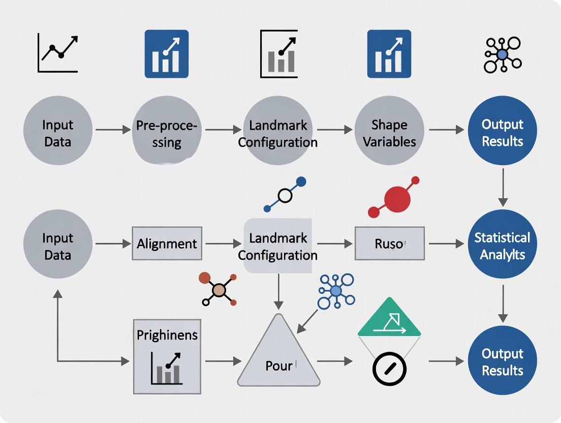
The following diagram illustrates the integrated analytical workflow for applying geometric morphometrics in parasite research and drug development:

Geometric morphometrics provides parasite researchers and drug development professionals with a rigorous quantitative framework for analyzing morphological structures. By implementing standardized protocols for landmark digitization, Procrustes superimposition, and multivariate statistical analysis, researchers can extract meaningful biological insights from subtle shape variations. The integration of these approaches into antimalarial drug development pipelines offers promising opportunities to identify morphological biomarkers of drug efficacy and understand parasite responses to therapeutic intervention at the structural level.

Application Notes

Functional Morphology of Attachment in Monogeneans

In Monogenean parasites, the haptor (a specialized posterior attachment organ) is a complex structure equipped with hardened sclerites and associated musculature that enables firm adhesion to host tissues. In Tetraonchus monenteron, a parasite of pike, the haptoral armature consists of ventral and dorsal pairs of anchors, a ventral bar, eight pairs of marginal hooks, and at least three pairs of accessory sclerites [6] [7]. These sclerites are operated by a sophisticated system of 14 muscles [6]. The dorsal anchors achieve a gaffing action primarily through the coordinated effort of extrinsic muscles and a transverse muscle that clamps them against the body wall [6] [7]. Conversely, the ventral anchors are stabilized in position by the transverse muscle and additional muscles inserting on the ventral bar and haptoral wall [6] [7]. This intricate musculoskeletal arrangement is a key taxonomic character and highlights the haptor's adaptation for securing the parasite to a dynamic, mobile host.

Shape Variation in Cymothoid Isopod Attachment Structures

In Cymothoid isopods, the shape of the attachment claws, known as dactyli, directly reflects their parasitic strategy and the functional demands of their specific microhabitat on the host fish [8]. Externally-attaching species (e.g., on the skin) are subject to greater hydrodynamic forces and possess dactyli that are relatively longer, thinner, and more needle-like, an adaptation for piercing flesh and resisting detachment [8]. In contrast, internally-attaching species (e.g., within the gill chamber or mouth) use their dactyli more for grasping hard structures like gill rakers; their dactyli are stouter, more recurved, and strengthened for a gripping function [8]. Geometric morphometric analyses confirm that parasite mode is the primary driver of this dactylus shape variation, with mouth-attaching species exhibiting greater shape variability than gill-attachers [8]. This ecomorphological pattern suggests that attachment structure morphology is a critical trait reinforcing host niche specialisation.

Insights from Parasite Community Structure

The study of parasite communities can provide indirect insights into the functional morphology of parasite structures by revealing patterns of host use and infestation. A study on the Cape elephant fish (Callorhinchus capensis) found a uniform parasite community structure across different host populations, indicating a highly interactive shark community with no significant population structure [9]. This suggests that parasites, and by extension their attachment mechanisms, are effectively dispersed across the entire host population. The parasite community was characterized by a low diversity of species, including a cestode (Gyrocotyle plana), two monogeneans (Callorhynchicotyle callorhynchi and Callorhinchicola multitesticulatus), an isopod (Anilocra capensis), and a leech (Branchellion sp.) [9]. The specific sites of attachment on the host (e.g., gills, spiral valve, external body surface) underscore the niche partitioning facilitated by specialized attachment structures [9].

Experimental Protocols

Protocol 1: Confocal Microscopy for Sclerite and Musculature Visualization

This protocol details the methodology for visualizing the hard sclerites and associated musculature of parasite attachment organs, as applied to the monogenean Tetraonchus monenteron [6] [7].

• 1. Sample Preparation and Fixation:

  • Collect parasite specimens from the host organism (e.g., gills of pike for T. monenteron).
  • Fix specimens in an appropriate fixative (e.g., 4% paraformaldehyde in phosphate-buffered saline) for several hours to preserve tissue structure.

• 2. Phalloidin Staining:

  • Permeabilize the fixed specimens using a detergent solution (e.g., 0.1% Triton X-100).
  • Incubate the specimens in a solution of phalloidin conjugated to a fluorophore (e.g, Alexa Fluor 488). Phalloidin specifically binds to F-actin, vividly staining the muscular architecture [6].
  • Perform several washes in a buffer to remove unbound stain.

• 3. Confocal Microscopy and Reflection Mode Imaging:

  • Mount the stained specimens on microscope slides.
  • Use a confocal laser scanning microscope to image the phalloidin-stained musculature.
  • Simultaneously, activate the reflection confocal mode to visualize the hardened sclerites (anchors, bars, hooks) based on their light-reflecting properties [6]. This allows for the simultaneous 3D rendering of both soft musculature and hard sclerites.

• 4. Data Analysis:

  • Use image analysis software to reconstruct the arrangement of muscles and sclerites.
  • Trace muscle pathways and their points of insertion on sclerites and the haptoral body wall to infer function [6] [7].

Protocol 2: Geometric Morphometric Analysis of Attachment Structures

This protocol outlines an outline-based geometric morphometric (GM) approach to quantify and analyze the shape of parasite attachment structures, as applied to cymothoid isopod dactyli and parasite eggs [10] [8].

• 1. Image Acquisition:

  • Capture high-resolution digital images of the attachment structures (e.g., dactyli, parasite eggs) using a camera mounted on a stereomicroscope. Ensure all specimens are photographed in a consistent orientation [8].

• 2. Landmarking:

  • Import images into specialized morphometric software (e.g., tpsDig2) [8].
  • Plot fixed landmarks on biologically homologous points (e.g., joint base, distal tip) [8].
  • Place semi-landmarks along curves and outlines between fixed landmarks to capture the overall shape geometry [8]. For example, a study on cymothoid dactyli used 3 fixed landmarks and 39 semi-landmarks to describe the shape [8].

• 3. Shape Analysis:

  • Perform a Generalized Procrustes Analysis (GPA) to superimpose landmark configurations, removing the effects of size, position, and orientation [10] [8].
  • The resulting Procrustes coordinates represent shape variables for subsequent statistical analysis.

• 4. Statistical Integration:

  • Use multivariate statistical tests (e.g., multivariate regression, discriminant analysis) to test hypotheses about the factors influencing shape, such as parasite mode, allometry, or host species [8].
  • Compare the Procrustes distances between groups to assess shape disparity [10] [8].
  • If data for multiple species is available, perform a Phylogenetic Generalized Least Squares (PGLS) analysis to account for the influence of shared evolutionary history [8].

Data Presentation

Table 1: Quantitative Summary of Haptoral Structures in Tetraonchus monenteron [6] [7]

Structure Type	Component	Quantity	Key Associated Muscles	Postulated Function
Anchors	Dorsal Anchor Pair	2	Extrinsic muscles (de, le1-3), muscles to body wall (daw1-2)	Gaffing, deep tissue penetration
	Ventral Anchor Pair	2	Transverse muscle (vat), muscles to ventral bar (vav1-3)	Stabilization, clamping
Bars	Ventral Bar	1	Connection point for muscles vav1-3	Structural support, muscle leverage
Marginal Hooks	Pairs	8	Protractor muscle (mp)	Fine-scale attachment & movement
Accessory Sclerites	Brace-shaped (brs)	≥ 2	Muscle bundles (brm)	Linking extrinsic muscles to dorsal anchors
	Flabellate (fs)	≥ 2	Muscles from dorsal anchor (daf1-2)	Muscle attachment
	Ball-shaped (bas)	≥ 2	Not specified	Unknown

Table 2: Factors Driving Dactylus Shape Variation in Cymothoid Isopods [8]

Factor	Effect on Dactylus Shape	Statistical Significance	Biological Interpretation
Parasite Mode (External vs. Internal)	Clear shape differences; external = longer, needle-like; internal = stouter, recurved	Primary driver (p < 0.05)	Functional adaptation to microhabitat (hydrodynamics vs. gripping)
Allometry (Size)	Significant for anterior (P1) dactyli; not significant for posterior (P7) dactyli	Anterior: SignificantPosterior: Not Significant	Shape changes with growth are more pronounced in the anterior appendage
Phylogeny	No clade-specific patterns of association with parasite mode	Not Significant	Parasite mode overrides evolutionary history (convergent evolution)

Mandatory Visualization

Diagram 1: Geometric Morphometric Workflow

Diagram 2: Haptor Musculoskeletal System

The Scientist's Toolkit

Table 3: Essential Research Reagents and Materials for Morphological Analysis of Parasite Structures

Research Reagent / Material	Critical Function	Application Example
Phalloidin-Fluorophore Conjugate	Selectively binds to filamentous actin (F-actin) in muscle fibers, enabling high-resolution visualization of the muscular architecture.	Staining the complex arrangement of 14 muscles operating the anchors in Tetraonchus monenteron [6] [7].
Confocal Laser Scanning Microscope	Allows for optical sectioning of tissues to generate 3D reconstructions; reflection mode can visualize hard, light-reflecting sclerites without staining.	Simultaneous imaging of phalloidin-stained musculature and reflective sclerites in a monogenean haptor [6].
Geometric Morphometric Software (e.g., tpsDig2)	Provides tools for digitizing biological landmarks and semi-landmarks on digital images for quantitative shape analysis.	Quantifying shape variation in the dactyli of cymothoid isopods using fixed landmarks and semi-landmarks [8].
Molecular Phylogenetic Tools (PCR, DNA sequencer)	Generates data to reconstruct evolutionary relationships among parasite species, allowing tests of shape evolution independent of phylogeny.	Conducting Phylogenetic Generalized Least Squares (PGLS) regression to account for shared ancestry in shape analysis [8].
TTP607	TTP607	Chemical Reagent
trans-Anol	trans-Anol, CAS:20649-39-2, MF:C9H10O, MW:134.17 g/mol	Chemical Reagent

The study of host-parasite co-evolution represents a cornerstone of evolutionary biology, providing critical insights into the dynamic interplay between species. Within this field, geometric morphometrics (GMM) has emerged as a powerful quantitative framework for analyzing how parasite attachment structures evolve in response to host-specific selective pressures. By quantifying shape variation using Cartesian coordinates of anatomically homologous landmarks, researchers can test hypotheses about the functional demands of different parasitic strategies and their evolutionary consequences. This protocol details the application of GMM to investigate how variation in parasite attachment structures reflects divergent evolutionary pathways and ecological specializations.

The recurved dactyli of cymothoid isopods and the haptoral anchors of monogenean flatworms serve as exemplary model systems. These structures are not merely taxonomic features but functional interfaces whose morphologies are fine-tuned by evolutionary processes. Research on cymothoid isopods has demonstrated clear morphological differences between externally-attaching and internally-attaching species, with shape variation correlating strongly with parasitic mode rather than shared ancestry [8]. Similarly, studies on Ligophorus cephali anchors have revealed significant phenotypic plasticity, suggesting host-driven plastic responses that facilitate host-switching and rapid speciation [11]. These findings underscore the value of GMM in unraveling the complex relationship between parasite form and function.

Key Concepts and Biological Foundations

Principles of Geometric Morphometrics in Parasitology

Geometric morphometrics differs fundamentally from traditional morphometric approaches by preserving the complete geometric configuration of anatomical structures throughout analysis. This methodology involves:

• Landmark-Based Analysis: Using two-dimensional or three-dimensional coordinates of biologically homologous points to capture shape information
• Procrustes Superimposition: A standardization procedure that removes differences in size, position, and orientation by centering shapes on the same point, scaling them to unit size, and rotating them to minimize least-squares distances between corresponding landmarks [12]
• Shape Space Construction: Creating multidimensional spaces where each point represents a unique shape configuration, allowing for statistical analysis of shape variation

The power of GMM lies in its ability to visualize shape differences directly through deformation grids, vector diagrams, and morphospace plots, providing intuitive representations of complex morphological variation.

Functional Morphology of Parasite Attachment Structures

Parasite attachment organs represent remarkable evolutionary adaptations that balance multiple functional demands:

• Attachment Security: Maintaining firm attachment against host defenses and environmental forces
• Resource Acquisition: Facilitating feeding while minimizing damage to host tissues
• Reproductive Capacity: Allowing for mating and reproduction while attached to the host

In cymothoid isopods, the recurved dactyli (hook-like appendages) on pereopods show distinct morphological specializations based on attachment location. Externally-attaching species, which face greater hydrodynamic forces, tend to have longer, more needle-like dactyli adapted for piercing flesh, while gill- and mouth-attaching species possess stouter, more recurved dactyli optimized for gripping host structures [8]. Similarly, in monogeneans like Ligophorus cephali, the dorsal and ventral anchors of the haptor exhibit different morphological gradients and functional specializations, with the ventral anchors typically responsible for firmer attachment [11].

Table 1: Functional Demands on Parasite Attachment Structures by Microhabitat

Parasite Group	Attachment Mode	Functional Challenges	Morphological Adaptations
Cymothoid Isopods	External (skin)	High hydrodynamic drag; host musculature penetration	Elongated, needle-like dactyli for deep tissue penetration
Cymothoid Isopods	Gill chamber	Limited space; delicate branchial tissues	Recurved, stout dactyli for clasping gill rakers
Cymothoid Isopods	Mouth cavity	Tongue/palate attachment; feeding interference	Stout, hook-shaped dactyli for anatomical "replacement"
Monogeneans (Ligophorus)	Gill filaments	Mucosal surface adherence; host immune response	Complex anchor/bar complexes with differential mobility

Research Reagent Solutions and Essential Materials

Table 2: Essential Research Tools for Geometric Morphometrics of Parasite Structures

Item/Category	Specific Examples	Function/Application
Specimen Collections	Curated museum collections; field-collected specimens	Source of morphological data; taxonomic verification
Imaging Equipment	Nikon DS-Fi1 camera; Nikon SMZ1500 stereoscopic microscope	High-resolution digital image capture for landmark digitization
Landmark Digitization Software	tpsDig2; StereoMorph R package	Precise placement of landmarks and semi-landmarks on digital images
Geometric Morphometric Analysis Software	MorphoJ; geomorph R package; CoordGen	Procrustes superimposition; statistical shape analysis; visualization
Molecular Phylogenetics Tools	PCR amplification; Cytochrome Oxidase I (COI) sequencing	Phylogenetic framework for comparative analyses
Statistical Packages	R with specialized packages (vegan, ape)	Multivariate statistical analysis; phylogenetic comparative methods

Experimental Protocol: Geometric Morphometric Analysis of Parasite Attachment Structures

Specimen Preparation and Imaging

• Specimen Sourcing and Curation:

  • Obtain parasite specimens from natural infestations or scientific collections
  • Ensure proper taxonomic identification using both morphological and molecular characters
  • For cymothoid isopods, focus on adult females to minimize sex-based variation [8]

• Standardized Imaging Protocol:

  • Mount specimens in consistent orientation to minimize projection artifacts
  • Use calibrated stereomicroscope with attached digital camera (e.g., Nikon DS-Fi1 on SMZ1500 microscope)
  • Capture high-resolution images of specific attachment structures (e.g., P1 and P7 pereopods in isopods; dorsal and ventral anchors in monogeneans)
  • Include scale bars in all images for size calibration
  • Maintain consistent lighting conditions and magnification across all specimens

Landmark Configuration and Digitization

• Landmark Selection Criteria:

  • Identify homologous points that can be reliably located across all specimens
  • Include Type I landmarks (discrete anatomical junctions), Type II landmarks (maxima of curvature), and Type III landmarks (extremal points)
  • For cymothoid dactyli, use a configuration of 3 fixed landmarks and 39 semi-landmarks along two curves [8]
  • Ensure the same number and sequence of landmarks for all specimens

• Semi-Landmark Placement:

  • Define curves between fixed landmarks using mathematical functions
  • Place semi-landmarks equidistantly along curves to capture outline geometry
  • For sliding semi-landmarks, implement algorithms that minimize bending energy or Procrustes distance [12]
  • Use software such as tpsDig2 or StereoMorph for standardized digitization

Data Processing and Shape Analysis

• Procrustes Superimposition:

  • Implement Generalized Procrustes Analysis (GPA) to align all landmark configurations
  • Remove non-shape variation through translation, scaling, and rotation
  • Generate Procrustes coordinates representing shape variables for statistical analysis
  • Calculate consensus (mean) shape as reference for visualization

• Statistical Analysis of Shape Variation:

  • Perform Principal Component Analysis (PCA) to identify major axes of shape variation
  • Conduct multivariate regression (e.g., Procrustes ANOVA) to test allometric effects
  • Implement discriminant analysis to assess group separability by parasitic mode
  • Apply phylogenetic comparative methods (e.g., phylogenetic GLS) to account for evolutionary relationships

Workflow for Geometric Morphometric Analysis of Parasite Structures

Data Analysis and Interpretation

Case Study: Cymothoid Isopod Dactyli

The application of GMM to cymothoid isopod dactyli reveals clear patterns of morphological adaptation:

Table 3: Shape Variation in Cymothoid Isopod Dactyli by Attachment Mode

Attachment Mode	Anterior Dactyli (P1) Shape	Posterior Dactyli (P7) Shape	Allometric Pattern	Functional Interpretation
Mouth-attachers	High shape variability; stout, recurved	Moderate variability; gripping morphology	Significant allometry	Adaptation to diverse intra-oral attachment sites
Gill-attachers	Intermediate shape; curved for raker clasping	Consistently recurved; strengthened	Moderate allometry	Optimization for branchial chamber environment
Skin-attachers	Elongated, needle-like; minimal curvature	Slender, piercing morphology	Non-significant allometry	Specialization for deep tissue penetration

Statistical analysis of 124 individuals across 18 species demonstrated that parasite mode explains a significant proportion of shape variation, with mouth-attaching species showing greater shape variability than gill- or skin-attaching species [8]. Phylogenetic comparative methods confirmed that these patterns reflect ecological specialization rather than shared evolutionary history.

Case Study: Monogenean Haptoral Anchors

Research on Ligophorus cephali haptoral anchors illustrates the value of GMM in detecting phenotypic plasticity:

• Dorsal and ventral anchors show similar gradients of overall shape variation, but dorsal anchors exhibit higher localized changes
• The dorsal anchor/bar complex demonstrates greater mobility than the ventral complex, suggesting functional differentiation
• Ventral anchors show less residual variation, indicating tighter developmental control, possibly due to their role in firm attachment
• High morphological integration between anchors reflects their concerted action during attachment
• The low genetic variation coupled with significant morphological variation suggests host-driven plastic responses rather than genetic differentiation [11]

Evolutionary Framework for Parasite Attachment Structure Morphology

Advanced Applications and Research Implications

Integration with Genomic Approaches

The combination of GMM with genomic methods provides unprecedented insights into co-evolutionary processes:

• Population Genomics: Studies on microsporidian parasites (Hamiltosporidium) of Daphnia magna demonstrate how demographic history and transmission mode shape genomic variation, which can be correlated with morphological changes in attachment structures [13]
• Phylogenetic Comparative Methods: Mapping morphological data onto molecular phylogenies enables discrimination between phylogenetic constraint and adaptive evolution in parasite attachment structures [8]
• Genotype-Phenotype Mapping: Identifying genetic loci associated with specific morphological variants can reveal the genetic architecture underlying attachment organ development

Implications for Drug and Vaccine Development

Understanding the functional morphology of parasite attachment interfaces has practical applications:

• Anti-Adhesion Therapies: Identifying morphological vulnerabilities in attachment mechanisms can inform strategies to disrupt host-parasite interfaces
• Vaccine Target Identification: Highly conserved attachment structures undergoing strong selective pressure may represent promising vaccine targets
• Drug Delivery Optimization: Knowledge of site-specific attachment morphologies can guide targeted delivery of chemotherapeutic agents

Troubleshooting and Technical Considerations

Common Methodological Challenges

• Landmark Homology: Ensuring true biological homology across diverse taxa requires careful anatomical study and may necessitate the use of semi-landmarks for complex curves
• Measurement Error: Conduct repeated digitization sessions to quantify and account for measurement error, which should be substantially smaller than biological variation of interest [14]
• Size Allometry: While Procrustes superimposition removes size, allometric effects on shape should be explicitly tested using multivariate regression [8]
• Phylogenetic Independence: Implement phylogenetic comparative methods to account for non-independence of related species

Sample Size Considerations

Determining adequate sample size depends on:

• The magnitude of shape differences between groups relative to within-group variation
• The number of landmarks and their capacity to capture biologically relevant shape information
• The complexity of the statistical analyses planned
• As a general guideline, studies of cymothoid isopods have successfully detected morphological differences with 5-10 specimens per species across 18+ species [8]

Geometric morphometrics provides a powerful, quantitative framework for investigating the functional morphology of parasite attachment structures and their role in host-parasite co-evolution. The protocols outlined here enable researchers to move beyond qualitative descriptions to test specific hypotheses about how ecological factors, evolutionary history, and functional demands shape parasite morphology. Through careful application of these methods—from standardized imaging and landmarking to sophisticated statistical analysis and phylogenetic comparison—we can decipher the complex relationship between form and function in parasitic organisms. The continued integration of GMM with genomic, ecological, and experimental approaches will further enhance our understanding of co-evolutionary dynamics and may inform novel strategies for parasite control.

Application Note

The study of morphological adaptation in parasites provides critical insights into host-parasite co-evolution and ecological specialization. Geometric morphometrics (GM) has emerged as a powerful alternative to traditional linear morphometrics, enabling a more nuanced and powerful analysis of shape by preserving the complete geometry of anatomical structures throughout the statistical analysis [15] [16]. This approach is particularly valuable for analyzing the sclerotized haptoral structures of monogenean flatworms, which are crucial for attachment and survival. In the genus Diplorchis, parasites that infect the urinary bladder of anurans, the haptoral anchors are not only taxonomically informative but also represent a model system to understand how host species and environmental factors drive morphological variation [17] [18]. This application note details a protocol for quantifying and interpreting shape variation in Diplorchis haptoral anchors, providing a framework for understanding morphological adaptation in parasites.

Key Findings from the Case Study

A recent study investigating six recorded and one unidentified species of Diplorchis in China revealed significant morphological variation driven by multiple factors [17] [18]. The key findings are summarized in the table below.

Table 1: Summary of Key Findings on Shape Variation in Diplorchis Haptoral Anchors

Analysis Level	Key Finding	Interpretation
Interspecific	Significant differences in anchor shape and size among the seven Diplorchis species.	Anchor morphology can serve as a reliable basis for species identification within the genus.
Intraspecific (Geographic)	Significant differences in anchor form, body size, and haptor size in the same species from different localities.	Habitat environment influences host biology/behavior, which in turn affects the parasite's attachment organ.
Intraspecific (Host-driven)	In two species from the same location, anchor and sucker size were not significantly different, but body and haptor size were.	Significant differences in anchor shape suggest that the attachment mechanism is species-specific and related to anchor shape variation.
Phylogenetic Signal	(Noted in related monogenean studies) Shape and size of haptoral anchors, particularly ventral ones, can show significant phylogenetic signal.	Common evolutionary history can be a major factor determining anchor form, alongside adaptive pressures [19] [20].

The study demonstrated that geometric morphometrics could successfully discriminate species and detect subtle shape variations linked to geographical isolation and host factors. The morphological variation in anchors is thus not random but is influenced by a combination of host species, habitat, and ecological environment, providing a basis for a deeper understanding of host-parasite interactions [17] [18].

Experimental Protocol

The following diagram illustrates the comprehensive workflow for a geometric morphometric analysis of monogenean haptoral anchors, from specimen preparation to statistical interpretation.

Detailed Step-by-Step Procedures

Specimen Collection and Preparation

• Source Parasites: Collect Diplorchis specimens from the urinary bladder of anuran hosts. The cited study sampled specimens from museum collections held at institutions like the School of Life Sciences, Yunnan Normal University [17].
• Selection Criteria: Carefully screen specimens and exclude any anchors that show apparent deformation, tears, or ruptures to ensure data quality. A final set of 82 specimens was used in the foundational study [17].
• Mounting: For imaging, mount the whole parasite body on a standard microscope slide to ensure the haptor and its anchors are correctly oriented and visible [18].

Image Acquisition

• Equipment: Use a high-quality light microscope (e.g., Olympus BX53) connected to a digital camera and imaging software (e.g., cellSens ver.2.2) [17] [18].
• Standardization: Capture images at a consistent magnification. Ensure the anchor is in clear focus and not obscured by other structures like eggs or host tissue.
• Data Management: To avoid data duplication, mark and photograph only one anchor (e.g., the right anchor) per specimen [18].

Landmark Digitization

This step converts morphological structures into quantitative data. Landmarks are homologous points that can be reliably identified across all specimens.

• Software: Input images into tpsUtil to create a TPS file. Then, use tpsDig2 to collect landmark coordinates [18] [21].
• Landmark Configuration: The protocol for Diplorchis used a combination of fixed landmarks and semi-landmarks [18]:
  • Six Fixed Landmarks: Precisely defined homologous points (e.g., tip of the hamuli, tip of the guard, tip of the handle) [18].
  • Fourteen Semi-landmarks: Placed along curves between fixed landmarks to capture outline geometry (e.g., from the most prominent point of the guard to the lowest point of the shaft) [18].
• Landmark Type Overview:

Table 2: Landmark Types in Geometric Morphometrics [21]

Type	Name	Description	Example
Type I	Anatomical Landmarks	Points of clear biological/anatomical significance.	Tip of the hamuli [18].
Type II	Mathematical Landmarks	Points defined by geometric properties (e.g., point of maximum curvature).	The base of the prominent crest [18].
Type III	Constructed Landmarks	Points defined by their relative position to other landmarks.	The midpoint between two other landmarks.

The following diagram illustrates the application of these landmark types on a schematic haptoral anchor.

Procrustes Superimposition and Statistical Analysis

• Generalized Procrustes Analysis (GPA): Import the landmark data into specialized software like MorphoJ. Perform GPA to remove the effects of size, position, and orientation by scaling, translating, and rotating landmark configurations. This creates a set of Procrustes shape coordinates for analysis [18] [21].
• Principal Component Analysis (PCA): Perform a PCA on the Procrustes coordinates to identify the major independent axes (Principal Components) of shape variation within the dataset. This helps visualize the main patterns of shape change and the distribution of different groups in a morphospace [18] [19].
• Canonical Variate Analysis (CVA): Use CVA to maximize the separation among pre-defined groups (e.g., species or populations). This is a powerful tool for testing hypotheses about group differences [18].
• Statistical Testing: Assess the significance of shape differences between groups using a permutation test (e.g., with 10,000 iterations, α = 0.05) [18].

The Scientist's Toolkit

Table 3: Essential Research Reagents and Software for Geometric Morphometrics

Item	Function/Description	Example Software/Version
Light Microscope with Camera	High-resolution imaging of sclerotized structures.	Olympus BX53 [17].
Image Management Software	Creates and manages TPS files from images.	tpsUtil (v1.82) [21].
Landmark Digitization Software	Collects 2D landmark coordinates from images.	tpsDig2 (v2.32) [18] [21].
Geometric Morphometrics Analysis Software	Performs Procrustes fitting, PCA, CVA, and visualization.	MorphoJ (v1.08) [18] [21].
Statistical Computing Environment	Advanced statistical analysis and custom scripting.	R (v4.3.2) with Momocs and dplyr packages [21].
Furfuryl hexanoate	Furfuryl hexanoate, CAS:39252-02-3, MF:C11H16O3, MW:196.24 g/mol	Chemical Reagent
Capryl alcohol-d18	Capryl alcohol-d18, CAS:69974-54-5, MF:C8H18O, MW:148.34 g/mol	Chemical Reagent

The Role of GM in Understanding Biogeographic Patterns and Evolutionary Constraints

Geometric morphometrics (GM) has emerged as a powerful quantitative method for analyzing biological shape, providing unprecedented insights into biogeographic patterns and evolutionary constraints. This approach utilizes geometric coordinates of morphological landmarks to statistically analyze shape variation and its relationship to biological, ecological, and evolutionary factors [22]. Within parasitology, GM offers a sophisticated toolkit for understanding how parasite attachment structures evolve in response to host specificity, environmental pressures, and geographical distribution [17] [8].

The application of GM to parasite research represents a significant advancement over traditional linear morphometrics by enabling researchers to visualize complex shape changes, separate size and shape variation, and statistically test hypotheses about evolutionary adaptation [17] [22]. This is particularly valuable for studying parasitic organisms where attachment organs are critical for host exploitation and survival, and where morphological variations often reflect adaptations to specific host environments and geographical contexts [17] [8].

Key Applications in Parasite Biogeography and Evolution

Analyzing Attachment Structure Evolution

The morphological variation of specialized attachment structures in parasites provides critical insights into evolutionary adaptations driven by host relationships and environmental factors. In monogenean flatworms of the genus Diplorchis, geometric morphometric analyses of haptoral anchors have revealed significant interspecific and intraspecific differences correlated with host species and geographical location [17]. These shape variations directly influence attachment mechanisms and reflect adaptive responses to ensure stable anchorage in different host environments.

Similarly, studies of cymothoid isopods have demonstrated that dactylus shape (hook-like appendages) strongly correlates with parasitic mode, where externally-attaching species exhibit differently shaped dactyli compared to gill- and mouth-attaching species [8]. This morphological variation reflects functional demands of attachment in different microhabitats and appears to be primarily driven by ecological factors rather than phylogenetic constraints, indicating convergent evolution in attachment mechanisms [8].

Resolving Biogeographical Patterns

GM approaches have proven valuable for elucidating biogeographical distributions and evolutionary relationships among parasite populations across different regions. Research on crane flies of the genus Ischnotoma utilized wing venation landmarks to successfully discriminate between subgenera from Neotropical and Australian regions, revealing clear morphological separations that correspond to geographical distributions [23]. The analysis demonstrated complete separation of three subgenera through Canonical Variate Analysis, providing insights into their evolutionary relationships and biogeographical history [23].

The application of GM has also revealed intraspecific geographical variations in parasite morphology. For instance, the same Diplorchis species collected from different localities exhibited significant differences in anchor form, body size, and haptor size, reflecting how different habitat environments affect host biological and behavioral activities, which subsequently influences parasite attachment structures [17].

Assessing Environmental Influences

Geometric morphometrics enables precise quantification of how environmental factors shape parasite morphology through both direct and host-mediated effects. Studies have shown that parasites from the same host species but different geographical locations can exhibit significant morphological divergence in their attachment structures, suggesting local environmental adaptation [17]. Interestingly, when two different parasite species inhabit the same geographical location, they may show no significant differences in anchor or sucker size, while still differing significantly in body size and haptor size, indicating complex environmental filtering mechanisms [17].

Table 1: Key Findings from Geometric Morphometric Studies of Parasites

Parasite Group	Biological Structure Analyzed	Key Finding	Evolutionary Implication
Diplorchis species (Monogenea) [17]	Haptoral anchors	Significant shape differences among species and between same species from different localities	Adaptation to host species and local environmental conditions
Cymothoid isopods [8]	Pereopod dactyli	Clear shape differences between externally-attaching and internally-attaching species	Functional adaptation to parasitic mode and microhabitat
Ischnotoma crane flies [23]	Wing venation	Complete separation of three subgenera using CVA	Biogeographical patterning and evolutionary relationships
Varroa destructor-infested bees [24]	Wing venation	96.4% separation between infested and control groups	Environmental stress effects on host morphology

Experimental Protocols and Methodologies

Landmark-Based Geometric Morphometrics Protocol

Objective: To quantify and analyze shape variation in parasite attachment structures or host morphological features affected by parasitism.

Materials and Equipment:

• Specimens (parasites or hosts)
• Stereomicroscope with calibrated digital camera
• Specimen preparation materials (slides, mounting medium)
• Computer with morphometric software (tpsSuite, MorphoJ, R with geomorph package)

Procedure:

• Specimen Preparation and Imaging

  • Fix and preserve specimens according to standard protocols for the target organisms
  • Mount specimens consistently to minimize orientation artifacts
  • Capture high-resolution digital images using standardized magnification and lighting conditions
  • Ensure all relevant structures are clearly visible and in focus

• Landmark Digitization

  • Select homologous landmarks that accurately capture the shape of the structure of interest
  • Define landmark types (Type I: discrete anatomical junctions; Type II: maxima of curvature; Type III: extreme points)
  • Use tpsDig2 software to plot coordinates for all landmarks across all specimens [8] [24]
  • Include semi-landmarks for curves and outlines where necessary [8]

• Generalized Procrustes Analysis (GPA)

  • Superimpose landmark configurations to remove effects of position, orientation, and scale
  • Rotate configurations to minimize Procrustes distance between corresponding landmarks
  • Obtain Procrustes coordinates representing shape variables for subsequent analysis

• Statistical Analysis of Shape Variation

  • Perform Principal Component Analysis (PCA) to identify major axes of shape variation
  • Conduct Canonical Variate Analysis (CVA) to test for group differences (e.g., by species, location, host)
  • Implement regression analysis to assess allometry (shape-size relationships)
  • Use thin-plate spline visualizations to illustrate shape changes [17] [23]

• Interpretation and Visualization

  • Generate deformation grids to visualize shape changes along significant axes
  • Create scatterplots of principal components or canonical variates
  • Statistically test hypotheses about group differences using MANOVA procedures
  • Correlate shape variables with ecological, geographical, or host factors

Figure 1: Workflow for landmark-based geometric morphometric analysis of parasite structures, showing key stages from specimen collection to results interpretation.

Case Study: Analysis of Monogenean Haptoral Anchors

Background: This protocol adapts methodology from studies of Diplorchis species to analyze shape variation in monogenean haptoral anchors in relation to host specificity and geographical distribution [17].

Specific Modifications:

• Focus on haptoral anchors as key attachment structures
• Include landmarks capturing anchor point, shaft curvature, and blade morphology
• Compare specimens from different host species and geographical locations
• Analyze both shape and size variables to assess allometric effects

Analytical Approach:

• Test for significant differences in anchor shape between species using CVA
• Assess correlation between geographical distance and morphological divergence
• Evaluate effect of host ecology on anchor morphology using multivariate regression
• Map shape changes onto phylogenetic hypotheses when available

The Scientist's Toolkit: Essential Research Reagents and Materials

Table 2: Essential Research Reagents and Materials for Parasite Geometric Morphometrics

Item	Specification	Application/Function
Imaging System	Stereomicroscope with digital camera (e.g., Nikon DS-Fi1, Olympus DP80) [8]	High-resolution image capture of parasite structures
Specimen Mounting	Microscope slides, coverslips, mounting medium	Consistent specimen orientation for imaging
Landmarking Software	tpsDig2 [8] [24]	Precise digitization of landmark coordinates
Morphometric Analysis Software	MorphoJ, tpsRelw, R with geomorph package [23]	Statistical shape analysis and visualization
Phylogenetic Analysis Tools	Molecular sequencing reagents, phylogenetic software	Contextualizing morphological variation within evolutionary framework
Reference Specimens	Voucher specimens from museum collections [23]	Ensuring taxonomic accuracy and morphological comparison
Cinnamyl azide	Cinnamyl Azide
Quadazocine mesylate	Quadazocine Mesylate|Opioid Receptor Antagonist	Quadazocine mesylate is a potent, non-selective silent antagonist at μ-, κ-, and δ-opioid receptors. For Research Use Only. Not for human or veterinary use.

Visualization Approaches for Shape Analysis

Visualizing Shape Deformation and Variation

Effective visualization is crucial for interpreting geometric morphometric results. The following approaches facilitate understanding of complex shape data:

Thin-Plate Spline Deformation Grids: These visualizations illustrate shape changes between specimens or groups by deforming a reference grid into a target configuration. They are particularly useful for showing how specific anatomical regions vary between groups [17].

Principal Component Scatterplots: Plots of specimen scores along major principal components reveal patterns of shape variation and grouping. Coloring points by factors such as species, geographical origin, or host type helps identify morphological trends [23].

Canonical Variate Plots: When testing a priori groupings, CVA plots show the maximum separation between groups, making them ideal for visualizing species differences or geographical variants [23].

Figure 2: Relationship between analytical steps and visualization methods in geometric morphometrics, showing how raw landmark data is transformed into interpretable visual outputs.

Data Analysis and Interpretation Framework

Statistical Framework for Hypothesis Testing

Robust statistical analysis is essential for drawing meaningful conclusions from geometric morphometric data. Key analytical approaches include:

Multivariate Analysis of Variance (MANOVA): Tests for significant differences in shape between predefined groups. In parasite studies, this might involve comparing attachment structures between species, populations from different geographical regions, or parasites from different host species [17] [24].

Regression Analysis: Assesses relationships between shape variables and continuous predictors such as size (allometry), geographical coordinates, or environmental variables. For example, studying how parasite attachment structures change with body size provides insights into developmental constraints [8] [23].

Partial Least Squares (PLS) Analysis: Examines covariation between shape data and other variable sets, such as ecological parameters or host traits. This approach is particularly useful for identifying coordinated changes between parasite morphology and host characteristics [17].

Integrating Geometric Morphometrics with Complementary Approaches

To fully understand biogeographic patterns and evolutionary constraints, GM should be integrated with other analytical approaches:

Molecular Phylogenetics: Combining shape analysis with molecular phylogenies helps distinguish between phylogenetic constraint and adaptive evolution in parasite morphology [8].

Environmental Data Analysis: Correlating shape variation with environmental variables (temperature, humidity, altitude) reveals selective pressures shaping parasite morphology across geographical gradients [17].

Host-Parasite Coevolution Analysis: Simultaneous analysis of host and parasite morphological traits identifies patterns of coevolution and adaptation in parasite attachment structures and host attachment sites [17] [8].

Geometric morphometrics provides a powerful framework for investigating biogeographic patterns and evolutionary constraints in parasite morphology. The protocols and applications outlined in this document demonstrate how GM approaches can reveal subtle shape variations in parasite attachment structures that reflect adaptations to host specificity, environmental conditions, and geographical distribution. By implementing standardized protocols for specimen preparation, landmark digitization, and statistical analysis, researchers can generate comparable data across studies and parasite taxa, advancing our understanding of how morphological evolution supports parasitic lifestyles across diverse biogeographic contexts.

From Specimen to Statistical Output: A Step-by-Step GM Protocol for Parasitology

Geometric morphometrics (GM) has revolutionized the quantitative analysis of biological forms, providing powerful tools for capturing and analyzing the shape of anatomical structures. Within parasitology, this approach is particularly valuable for investigating the intricate sclerotized structures of parasites, such as the haptoral anchors of monogeneans. These structures are not only critical for taxonomic identification but also reflect adaptations to specific hosts and environments [17]. Establishing a robust, reproducible workflow for imaging, digitization, and software selection is therefore fundamental to generating high-quality, comparable data. This document outlines application notes and detailed protocols for integrating geometric morphometrics into parasitology research, providing a structured guide for researchers, scientists, and drug development professionals engaged in the morphological analysis of parasites.

The Scientist's Toolkit: Essential Software and Research Reagents

A successful GM workflow relies on a combination of specialized software for image processing, digitization, and statistical analysis, alongside standard laboratory reagents for specimen preparation. The table below summarizes the core digital toolkit and key reagents used in the preparation of parasite specimens for morphometric analysis.

Table 1: Key Research Reagent Solutions for Parasite Specimen Preparation

Item Name	Function/Application in GM Workflow
Sclerotized Stains	Selective staining of chitinous structures (e.g., haptoral anchors, hooks) to enhance contrast for imaging.
Clearing Agents	Rendering soft tissues translucent to enable clear visualization of embedded sclerites without dissection.
Polyvinyl Lactophenol	A common mounting medium that simultaneously clears, fixes, and preserves parasite specimens on microscope slides.
Neutral Buffered Formalin	Standard fixative for preserving the structural integrity of collected parasite specimens prior to staining and mounting.
(Rac)-Pregabalin-d10	(Rac)-Pregabalin-d10|High-Quality Isotopically Labeled Standard
Anticancer agent 30	Anticancer Agent 30|Research Compound|RUO

Table 2: Core Software Toolkit for Geometric Morphometrics Analysis

Software/Category	Specific Examples	Primary Function in GM Workflow
Image Processing	GM (GraphicsMagick) via Node.js, ImageJ	Batch processing (contrast, transparency), scaling, and orientation standardization of specimen images [25] [26].
Digitization & Landmarking	tpsDig2, MorphoJ	Defining and recording 2D/3D coordinates of homologous landmarks on digital images.
Statistical Shape Analysis	MorphoJ, R (geomorph package)	Performing Procrustes superimposition, PCA, MANOVA, and visualizing shape changes.

Experimental Protocols for Parasite Structure Analysis

Protocol: Specimen Preparation and Image Acquisition of Monogenean Haptoral Anchors

This protocol is adapted from methodologies used in contemporary studies of Diplorchis species and other monogeneans, focusing on generating consistent, high-quality images for landmarking [17].

Materials:

• Fixed monogenean specimens (e.g., from host urinary bladder or gills)
• Microscope slides and coverslips
• Polyvinyl lactophenol or equivalent mounting medium
• Compound microscope with camera system (calibrated for scale)
• Image capture software

Methodology:

• Specimen Selection: Select specimens with no apparent deformation, tears, or ruptures in the haptoral structures. This is critical for accurate shape representation [17].
• Mounting: Place the specimen in a drop of polyvinyl lactophenol on a microscope slide. Carefully position the specimen to ensure the haptor and its anchors lie flat and are fully extended. Gently lower a coverslip, avoiding lateral movement that could distort structures.
• Curing: Allow the mounted slide to cure for 24-48 hours to stabilize the specimen and ensure the medium has hardened.
• Image Acquisition: Using a compound microscope with a calibrated camera, capture high-resolution micrographs of the haptoral anchors.
  • Use consistent magnification across all specimens.
  • Ensure the focal plane captures the maximum two-dimensional outline of all anchor components.
  • Include a scale bar within each image frame for subsequent size calibration during digitization.
  • Save images in a lossless format (e.g., TIFF, PNG) to preserve data integrity.

Protocol: Image Pre-processing with GraphicsMagick (GM)

Automated pre-processing ensures uniformity in image quality, which reduces batch effects and facilitates more accurate landmark placement.

Materials:

• Directory of raw specimen images
• Node.js environment with the gm package installed [25] [26]

Methodology:

• Batch Contrast Enhancement: Run a script to standardize image contrast. The contrast() function in GM allows for enhancement or reduction of contrast using a multiplier value [26].

• Background Standardization: Use the transparent() function to remove or unify background colors, creating a consistent backdrop that improves landmark visibility [25].
• Image Scaling: Use GM's resize() function to scale all images to a uniform pixel dimension based on the known scale bar, ensuring all subsequent measurements are comparable.

Protocol: Landmarking and Data Generation

This protocol details the process of converting morphological structures into quantitative shape data.

Materials:

• Pre-processed and scaled specimen images
• Digitization software (e.g., tpsDig2)

Methodology:

• Landmark Definition: Define a set of Type I (homologous anatomical points) and Type II (extremes of maximum curvature) landmarks on the haptoral anchor. For a monogenean anchor, this typically includes the point of insertion, the tip of the root, and the point of maximum curvature along the shaft and blade [17].
• Landmark Digitization:
  • In tpsDig2, open the image file and sequentially place landmarks according to the defined scheme.
  • Ensure the order of landmark placement is consistent for every specimen.
  • Repeat the process for all specimens in the dataset.
• Data File Creation: The software will generate a TPS file containing the Cartesian coordinates (x, y) of all landmarks for all specimens. This file is the primary data input for subsequent statistical shape analysis.

Workflow Visualization and Logical Pathway

The entire process, from specimen collection to statistical insight, can be visualized as a sequential workflow. The following diagram, generated using Graphviz and adhering to the specified color palette, outlines the logical pathway and critical decision points.

Diagram Title: Geometric Morphometrics Workflow for Parasitology

Application in Parasite Research: A Case Study

The power of this GM workflow is exemplified by research on the genus Diplorchis, monogeneans parasitizing the urinary bladder of anurans. A 2025 study utilized geometric morphometrics to analyze the haptoral anchors of six Diplorchis species and one unidentified species [17].

Key Findings and Workflow Application:

• Species Discrimination: Geomorphometric analyses revealed significant interspecific differences in anchor shape and size, establishing anchor morphology as a reliable character for species identification within the genus [17]. This addresses the challenge of species identification when molecular data from older specimens are unavailable.
• Environmental Adaptation: The study documented significant intraspecific differences in anchor form, body size, and haptor size in the same parasite species collected from different geographic localities. This suggests that environmental factors and host ecology can drive morphological variation, potentially reflecting an adaptive response to ensure stable attachment in different host populations [17].
• Attachment Mechanics: The significant differences in anchor shape among species suggest a relationship between morphological variation and the underlying attachment mechanism, providing insights into host-parasite interactions at a functional level [17].

This case study demonstrates how a rigorously applied GM workflow can move beyond simple description to address complex questions about systematics, adaptation, and functional morphology in parasitology.

Geometric morphometrics (GM) has revolutionized the quantitative analysis of biological forms, proving particularly valuable in parasitology for distinguishing species and investigating host-parasite interactions. The analysis of parasite sclerites, such as the haptoral anchors of monogeneans, relies heavily on the precise digitization of homologous points. This application note delineates the critical distinction between traditional landmarks and semi-landmarks, providing a structured framework for selecting the appropriate approach in morphometric studies of parasite sclerites. We detail experimental protocols, provide a comparative analysis of quantitative data, and list essential research reagents, all framed within the context of advanced parasitic research.

In geometric morphometrics, landmarks are defined as discrete, homologous points that are biologically comparable across all specimens in a study. For parasite sclerites, examples include the precise tip of a hamulus or the point of bifurcation of a hook root [27]. These points represent true biological homologues. However, many biologically significant structures, such as the curved shafts of anchors or smooth margins of sclerites, lack a sufficient number of such discrete points to capture their form adequately.

Semi-landmarks are points used to quantify the geometry of these curves and surfaces [28]. They are not considered homologous in their initial placement but are made mathematically comparable through algorithms that slide them along a tangent direction or surface to minimize a bending energy or Procrustes distance against a mean reference form [29]. This process allows for the dense sampling of morphology between the fixed landmarks, enabling a comprehensive analysis of shape.

The choice between these methods is not merely technical; it directly influences the biological interpretation of results. Analyses based on semi-landmarks are considered "approximations of reality that require cautious interpretation" [28], as their locations can be influenced by the chosen algorithm and their density.

Theoretical Foundation and Decision Framework

The core of the landmark versus semi-landmark choice rests on the availability of homologous points and the research objective.

When to Use Traditional Landmarks

• Structures with abundant homologies: Sclerites with numerous distinct anatomical features (e.g., notches, tips, intersections) are well-suited for landmark-only analysis.
• Focus on discrete points of homology: When the research question specifically concerns the variation in the relative positions of known, developmentally conserved structures.
• Studies requiring minimal algorithmic influence: To avoid potential biases introduced by sliding algorithms, a landmark-only approach is more conservative.

When to Incorporate Semi-Landmarks

• Analyses of curves and outlines: The curved shafts of anchors, marginal hooks, or the overall outline of a sclerite are prime candidates for semi-landmarks [30].
• Dense sampling of form: When the research aims to capture the "overall form" of a sclerite beyond a few discrete points, semi-landmarks "increase the density of the shape information" [28].
• Structures with few true landmarks: This is a common scenario in parasitology, where sclerites may offer only a handful of unambiguous landmarks, making semi-landmarks essential for a powerful geometric analysis [28].

Table 1: Decision Matrix for Landmark and Semi-Landmark Application in Sclerite Analysis

Research Scenario	Recommended Approach	Rationale
Comparing specific hook tip morphology between species	Traditional Landmarks	Focuses analysis on discrete, homologous points of functional significance.
Quantifying shape variation of a curved anchor shaft	Semi-Landmarks	Allows for the quantification of continuous curvature that lacks discrete homologies.
Comprehensive analysis of entire haptoral anchor form	Combined Approach (Landmarks + Semi-Landmarks)	Fixed landmarks define core homologies; semi-landmarks capture the intervening geometry [30].
Ontogenetic studies of sclerite growth	Combined Approach	Tracks growth of specific landmarks while capturing allometric changes in overall shape.

Experimental Protocols for Sclerite Morphometrics

Protocol 1: Isolation and Preparation of Haptoral Sclerites

Accurate morphometric analysis requires cleanly isolated sclerites free from obscuring soft tissue.

• Sample Collection: Fix parasites removed from the host in 70% ethanol for morphological study or 96% ethanol for molecular analysis and subsequent sclerite isolation [31].
• Digestion of Soft Tissue:
  • Place individual parasites on a polylysine-coated or concavity slide to prevent loss of minute sclerites.
  • Apply a digestion buffer. One effective buffer contains Tris-HCl, EDTA, Sodium Dodecyl Sulphate (SDS), and proteinase K as the active enzyme [31].
  • Incubate until the soft tissue is sufficiently digested, leaving the chitinous sclerites intact.
• Washing and Mounting: Carefully wash the digested material with distilled water to remove buffer residues. Mount the cleaned sclerites on a stub for Scanning Electron Microscopy (SEM) or on a slide for light microscopy.

Protocol 2: Data Acquisition and Digitization

This protocol covers the process from image capture to point digitization.

• Imaging: Capture high-resolution images of the isolated sclerites using a calibrated light microscope or SEM.
• Defining the Landmark Schema:
  • Identify a set of fixed landmarks that are unambiguously homologous across all specimens (e.g., the tip of the anchor, the base of the root).
  • Define curves between these fixed landmarks to be sampled with semi-landmarks. For instance, place a curve along the ventral root and another along the dorsal root [27].
• Digitization:
  • Digitize all fixed landmarks.
  • Place semi-landmarks equidistantly along the pre-defined curves. Software such as tpsDig2 or MorphoJ is commonly used for this process. The number of semi-landmarks should be consistent for all specimens.

Protocol 3: Sliding Semi-Landmarks and Statistical Analysis

This step makes semi-landmarks comparable for statistical shape analysis.

• Sliding Semi-Landmarks: Use geometric morphometric software (e.g., tpsRelw, geomorph R package) to slide the semi-landmarks. The two primary criteria are:
  • Minimize Bending Energy: Assumes the change between forms requires minimal deformation energy.
  • Minimize Procrustes Distance: Slides points to minimize the overall Procrustes distance among specimens [29].
• Generalized Procrustes Analysis (GPA): Superimpose the entire configuration of landmarks and slid semi-landmarks to remove the effects of position, orientation, and scale.
• Statistical Analysis: Analyze the Procrustes coordinates using multivariate statistics like Principal Component Analysis (PCA) to visualize major shape trends, or Discriminant Function Analysis to test for shape differences between pre-defined groups (e.g., species, populations) [17].

The following workflow diagram visualizes the complete process from specimen preparation to data analysis:

Data Presentation and Comparative Analysis

The application of these methods in parasitology has yielded significant insights. A study on Diplorchis species demonstrated that geometric morphometrics of haptoral anchors could reveal significant interspecific differences, supporting species identification [17]. Furthermore, the same study found intraspecific shape variation correlated with geographical location, highlighting the influence of environmental factors.

Table 2: Quantitative Comparison of Landmark Types for Parasite Sclerite Analysis

Characteristic	Traditional Landmarks	Semi-Landmarks
Basis of Homology	Developmental/Evolutionary homology [28]	Algorithmic point correspondence [28]
Ideal for Quantifying	Discrete points (tips, junctions)	Curves, outlines, surfaces
Data Density	Low (limited by number of homologies)	High (user-defined density) [30]
Influence of Method	Low	High (varies with algorithm and density) [28]
Primary Analysis Software	tps series, MorphoJ, R (geomorph)	tps series, MorphoJ, R (geomorph)
Role in Sclerite Studies	Core homologous framework; tracking specific points	Capturing overall form and curvature

The Scientist's Toolkit: Research Reagent Solutions

Successful geometric morphometric analysis of parasite sclerites depends on specific laboratory materials and reagents.

Table 3: Essential Research Reagents and Materials for Sclerite Morphometrics

Item	Function/Application	Example/Brief Explanation
Ethanol (70%, 96%)	Parasite fixation and preservation. 96% ethanol is preferred for specimens destined for molecular analysis or sclerite isolation.	Preserves sclerites without excessive hardening that can cause brittleness [31].
Digestion Buffer	Enzymatic removal of soft tissue to isolate sclerites.	Contains Tris-HCl, EDTA, SDS, and proteinase K to digest tissue while leaving chitinous sclerites intact [31].
Polylysine-coated Slides	Adhesive slides to prevent loss of microscopic sclerites during digestion and washing.	Creates a positively charged surface that binds cells and structures, minimizing sample loss [31].
Glycerine Ammonium Picrate (GAP)	A mounting medium for temporary or semi-permanent slides for light microscopy.	Used to clear and mount whole parasites for initial morphological examination and sclerite measurement [31].
Geometric Morphometric Software	For digitizing, sliding, and analyzing landmark data.	Essential tools like tpsDig2, MorphoJ, and the geomorph package in R form the computational backbone of the analysis.
Iloprost-d4	Iloprost-d4, MF:C22H32O4, MW:364.5 g/mol	Chemical Reagent
N,3-diethylaniline	N,3-diethylaniline, MF:C10H15N, MW:149.23 g/mol	Chemical Reagent

The strategic selection of landmarks and semi-landmarks is fundamental to robust geometric morphometric analysis of parasite sclerites. Traditional landmarks provide the foundational framework of homology, while semi-landmarks empower researchers to capture and quantify the continuous morphological variation of curves and surfaces. By adhering to the detailed protocols and decision frameworks outlined in this application note, researchers can effectively leverage these powerful tools. This approach facilitates a deeper understanding of parasite taxonomy, evolution, and host-parasite interactions, generating high-quality, quantitative data for a broader thesis in parasitology.

Geometric morphometrics (GM) is a powerful suite of methods for quantitatively analyzing biological shapes. In parasite research, the morphology of attachment structures often reflects parasitic strategy and niche specialization. Traditional linear measurements fail to capture the full complexity of shape, whereas GM allows researchers to statistically quantify and visualize subtle shape variations that are critical for understanding host-parasite interactions [8] [32]. This protocol focuses on two core GM techniques: Procrustes Superimposition, which separates pure shape from size, orientation, and position, and Principal Component Analysis (PCA), which identifies major patterns of shape variation within a dataset [33] [34]. When integrated, these techniques provide a robust framework for identifying morphological adaptations, such as the differences in hook-like dactyli between externally- and internally-attaching cymothoid isopods [8]. This document provides detailed application notes and protocols for implementing these techniques within a parasite morphology research pipeline.

Theoretical Foundations

Procrustes Superimposition

Procrustes superimposition is the foundational step in GM for obtaining "shape coordinates." Raw landmark coordinates collected from specimens contain non-shape information related to their size, position in space, and orientation. The goal of Procrustes analysis is to remove these confounding factors so that the resulting coordinates represent shape per se [33] [32]. This is achieved through a three-step process:

• Translation: All landmark configurations are translated to a common centroid, typically the origin (0,0) of a coordinate system.
• Scaling: Configurations are scaled to a standard size, known as unit centroid size. Centroid size is computed as the square root of the sum of squared distances of all landmarks from their centroid.
• Rotation: Configurations are rotated until the sum of squared distances between corresponding landmarks is minimized (the "least squares" criterion) [33].

The resulting Procrustes coordinates describe shape independently of size, position, and rotation, making them suitable for subsequent multivariate statistical analysis [33].

Principal Component Analysis (PCA)

PCA is a dimensionality reduction technique used to emphasize variation and identify strong patterns in a dataset [35]. In the context of GM, PCA is applied to Procrustes-aligned coordinates to simplify the interpretation of shape variation [33].

How PCA Works:

• Objective: To create new variables, called Principal Components (PCs), which are weighted sums (linear combinations) of the original shape variables [34].
• Variance Maximization: The first principal component (PC1) is the axis (direction) through the data that accounts for the maximum possible variance. The second component (PC2) is orthogonal to PC1 and accounts for the next greatest amount of remaining variance, and so on [36] [37].
• Mathematical Basis: PCA is performed by computing the eigenvectors and eigenvalues of the covariance (or correlation) matrix of the data. Eigenvectors define the directions of the new principal components, while eigenvalues indicate the amount of variance each PC explains [34] [36].

When applied to shape data, PCA produces a low-dimensional summary—such as a 2D or 3D scatter plot—where observations can be visualized, and trends, clusters, or outliers can be identified [34] [37]. The shape changes associated with each PC can be visualized as deformations of the original landmark configuration, providing direct biological interpretation [33].

Integrated Workflow: From Specimens to Shape Analysis

The following diagram illustrates the complete analytical pipeline, integrating specimen preparation, data digitization, Procrustes superimposition, and Principal Component Analysis.

Experimental Protocols

Protocol 1: Landmark Digitization and Procrustes Superimposition

This protocol is adapted from studies on parasite attachment structures [8] and nasal cavity morphology [38], which provide robust models for shape analysis.

I. Specimen Preparation and Image Acquisition

• Fixation and Storage: Preserve parasite specimens in 70-75% ethanol. For delicate structures, consider critical point drying to minimize deformation.
• Image Capture: Use a stereomicroscope (e.g., Nikon SMZ1500) fitted with a high-resolution digital camera (e.g., Nikon DS-Fi1). Ensure consistent magnification and orientation for all specimens. Capture multiple images if structures are three-dimensional.
• Quality Control: Ensure homogeneous illumination and that all relevant morphological features are in clear focus.

II. Landmark Digitization Landmarks are biologically homologous points that can be reliably identified across all specimens [39]. The choice of landmark type is critical.

• Fixed Landmarks: Identify precise anatomical loci (e.g., "the medial junction of the dactylus with the propodus" in isopods) [8]. Digitize 10-20 fixed landmarks, depending on structure complexity [38] [8].
• Semi-Landmarks: For curves and surfaces without discrete homologous points, place semi-landmarks. In a study on nasal cavities, 200 sliding semi-landmarks were used to capture the contour of the region of interest [38]. These are later "slid" during Procrustes analysis to minimize bending energy and establish geometrical homology [38] [32].
• Software: Use specialized software such as tpsDig2 [8] or Viewbox [38].
• Repeatability Assessment: To ensure data reliability, have the same operator digitize a subset of specimens twice and a second operator digitize them once. Quantify agreement using Lin’s Concordance Correlation Coefficient (CCC); values >0.90 indicate excellent repeatability [38].

III. Generalized Procrustes Analysis (GPA) GPA aligns all landmark configurations using the steps outlined in Section 2.1.

• Software Implementation: This can be performed in R using the geomorph package [38] or in other morphometric software like MorphoJ.
• Output: The output is a set of Procrustes coordinates for each specimen, which are now directly comparable as they contain only shape information [33].

Table 1: Landmark Types and Definitions in Geometric Morphometrics

Landmark Type	Definition	Example from Parasite Research	Key Consideration
Type I (Anatomical)	Discrete juxtapositions of tissues (e.g., bone sutures).	Junction of sclerotized structures in arthropod appendages.	Most reliable but often limited in number.
Type II (Maximum Curvature)	Points of maximum local curvature.	Tip of a hook or claw in parasite attachment structures.	Abundant but require careful definition.
Type III (Extreme Points)	Extremal points or endpoints of structures.	Extremities of elongated structures.	Can be less reliable than Type I/II.
Semi-Landmarks	Points placed on curves and surfaces to quantify outlines.	Outline of a dactylus in cymothoid isopods [8].	Must be slid during Procrustes analysis to establish homology.

Protocol 2: Principal Component Analysis of Shape Data

This protocol details how to perform PCA on Procrustes-aligned coordinates to extract and interpret major shape patterns.

I. Data Input and Pre-processing

• Input Data: Use the matrix of Procrustes coordinates generated from Protocol 1.
• Data Centering: The data is already centered by the Procrustes process (mean shape is at the origin). No further standardization is typically needed for shape coordinates.

II. Performing PCA

• Software Execution: In R, use the prcomp() function [34] or the PCA function within the FactoMineR package [38]. The analysis decomposes the shape variance into orthogonal principal components.
• Output Extraction: The key outputs are:
  • Scores: The new coordinates of each specimen in the principal component space [34].
  • Loadings (Eigenvectors): The weights that show how much each original landmark coordinate contributes to each PC [37].
  • Eigenvalues: The amount of total variance explained by each PC.

III. Determining the Number of Significant Components Select the number of PCs to retain for further analysis using these criteria:

• Scree Plot: Plot the eigenvalues in descending order. The "elbow" point, where the slope of the curve sharply levels off, indicates the number of meaningful components [38] [36].
• Cumulative Variance: Retain enough PCs to explain a pre-determined percentage of total variance (e.g., 80-95%) [40].
• Kaiser Criterion: Retain components with eigenvalues greater than 1 (more common in factor analysis but sometimes applied to PCA) [40].

IV. Visualization and Interpretation

• Score Plots: Create scatter plots of PC1 vs. PC2 (and higher PCs if needed) to visualize specimen clustering, trends, and outliers [34] [37].
• Shape Visualization: Use software to visualize the shape changes associated with the extremes (e.g., -0.1 and +0.1 units) of each PC. This is often shown as deformation grids or vectors from the mean shape [33].
• Biplots: Superimpose loadings (as vectors) onto a score plot to interpret which original variables (landmarks) are driving the separation along the PCs [34].

Table 2: Key Outputs of a PCA on Shape Data and Their Interpretation

PCA Output	Description	Interpretation in Shape Analysis
Scores	Coordinates of specimens in the new PC space.	Used in scatter plots to identify groups (morphotypes), clusters, or outliers. A specimen's score indicates its placement along a major axis of shape variation.
Loadings	Weightings of the original variables (landmark coordinates) on the PCs.	Reveal which specific landmarks are moving the most to create the shape variation described by a PC. High loadings indicate influential landmarks.
Eigenvalues	Amount of variance captured by each PC.	Determine the importance of each PC. A scree plot of eigenvalues helps decide how many PCs to retain.
Explained Variance (%)	The proportion of total shape variance accounted for by each PC.	PC1 explains the most variance, PC2 the second most, etc. The cumulative percentage indicates how much total information is retained in the reduced dimensions.

Application in Parasite Morphology Research: A Case Study

The analysis of attachment structures (dactyli) in cymothoid isopods provides an excellent example of applying these techniques in parasite research [8].

Background: Cymothoid isopods are obligate fish ectoparasites that attach in distinct regions (mouth, gills, skin). The shape of their hook-like dactyli is critical for attachment and survival.

Method Application:

• Landmarking: 39 semi-landmarks were used to describe the curves of the dactylus between three fixed landmarks [8].
• Procrustes & PCA: After Procrustes alignment, PCA was performed on the shape variables.
• Results: PCA revealed clear shape differences between dactyli of externally-attaching and internally-attaching (gill/mouth) parasites. This variation was linked to the functional demands of their respective microhabitats, supporting the hypothesis that attachment morphology is a key adaptive trait [8].

The following diagram conceptualizes how PCA transforms complex, correlated landmark data into interpretable patterns of shape variation.

The Scientist's Toolkit: Essential Reagents and Materials

Table 3: Research Reagent Solutions for Geometric Morphometrics

Item Name	Function/Application	Example Specifications/Notes
Ethanol (70-75%)	Specimen preservation and fixation.	Prevents tissue degradation and deformation. Higher concentrations can make specimens brittle.
Glycerol	Temporary mounting medium for microscopy.	Helps clear tissues for better visualization of internal structures.
Critical Point Dryer	Sample preparation for delicate structures.	Preserves 3D structure by replacing liquid with gas without surface tension damage.
High-Resolution Camera	Image acquisition for digitization.	e.g., Nikon DS-Fi1, mounted on a stereomicroscope [8].
Digitizing Software	Placing landmarks on digital images.	tpsDig2, Viewbox 4.0 [38] [8].
Statistical Software with GM Packages	Data analysis (Procrustes, PCA, visualization).	R with packages geomorph, FactoMineR [38]; MorphoJ.
D-Proline, 1-formyl-	D-Proline, 1-formyl-, CAS:899900-53-9, MF:C6H9NO3, MW:143.14 g/mol	Chemical Reagent
C18H12N6O2S	C18H12N6O2S Research Chemical|Supplier	High-purity C18H12N6O2S for research use only (RUO). Explore its applications in medicinal chemistry and drug discovery. Not for human or veterinary use.

Geometric morphometrics (GMM) has emerged as a powerful quantitative tool for the analysis of biological shape, demonstrating exceptional accuracy in the identification of medically significant parasites and arthropods. This application note details the protocols and analytical frameworks for implementing GMM in diagnostic contexts, where it has been reported to achieve 94.0–100.0% identification accuracy [41] [42] [43]. Unlike conventional diagnostic methods that often rely on subjective morphological assessments, GMM utilizes the statistical analysis of landmark coordinates to quantify subtle shape variations that are often imperceptible to the human eye. When framed within a broader research thesis on parasite morphology, this approach provides a reproducible, cost-effective, and high-throughput alternative to molecular techniques like DNA barcoding, offering a significant advancement for taxonomic resolution and species discrimination in clinical and field settings [41] [44].

Performance Data: GMM vs. Alternative Diagnostic Techniques

The following table summarizes the performance of GMM alongside other state-of-the-art diagnostic techniques for parasite and arthropod identification [41] [42] [43].

Table 1: Comparison of Advanced Diagnostic Techniques for Medical Parasites and Arthropods

Technique	Principle	Reported Accuracy/Precision	Key Advantages	Key Limitations
Geometric Morphometrics (GMM)	Statistical analysis of landmark-based shape patterns [12] [14].	94.0% - 100.0% [41] [42] [43]	High accuracy; no costly reagents; results visually interpretable [41] [44].	Requires homologous landmarks; limited species coverage in databases [41].
DNA Barcoding	Analysis of standardized short genetic sequences.	~95.0% [41] [42] [43]	High discriminatory power at species level.	Requires costly reagents and equipment; complex sample preparation [41].
Artificial Intelligence (AI)	Image analysis using trained deep learning algorithms [45].	98.8% - 99.0% [41] [42] [43]	Very high precision; potential for full automation.	Requires large, annotated datasets and significant computational resources [45].
Conventional Microscopy	Visual examination of specimens.	Variable; often lower sensitivity and specificity [42] [43]	Low cost; widely available.	Time-consuming; labor-intensive; requires skilled technicians; subjective interpretation [41] [42].

Detailed Experimental Protocol for GMM Analysis

This protocol provides a step-by-step guide for a typical GMM analysis, from data collection to statistical interpretation, adaptable for various parasite structures such as insect heads, pronota, or helminth sclerites [12] [14] [44].

Specimen Preparation and Image Acquisition

• Specimen Mounting: Fix and mount specimens (e.g., whole arthropods, parasite eggs, or morphological structures) consistently to minimize distortion.
• Image Capture: Use a high-resolution scanner (e.g., 300 dpi or higher) or a digital microscope camera to capture digital images of all specimens under identical lighting and magnification conditions [14]. Ensure the structure of interest is in the same orientation (e.g., dorsal view) across all images.

Landmark Digitization

• Landmark Definition: Define a set of homologous anatomical points (landmarks) that can be reliably identified across all specimens. The same number and type of landmarks must be digitized on every specimen in the same order [12]. Examples include vein intersections on insect wings, tips of mouthparts, or specific points on parasite egg shells.
• Software for Digitization: Use specialized software for landmark placement. The StereoMorph package in R provides a user-friendly interface for digitizing 2D landmarks and curves [12].
• Data Structure: The raw data is typically stored in a 3D array format: p (landmarks) × k (dimensions; 2 for 2D) × n (specimens) [12].

Procrustes Superimposition and Shape Variable Extraction

This critical step removes the effects of size, position, and orientation, isolating pure shape information.

• Procedure: Perform a Generalized Procrustes Analysis (GPA) using the gpagen() function in the geomorph R package [12]. This process consists of:
  • Centering: Translating all specimens so their centroids (geometric centers) overlap.
  • Scaling: Scaling all specimens to a unit centroid size.
  • Rotation: Rotating specimens to minimize the Procrustes distance (the sum of squared distances between corresponding landmarks) among them [12].
• Output: The analysis produces Procrustes shape coordinates, which are the aligned coordinates used for all subsequent statistical analyses. The geomorph.data.frame function is used to create a data object that combines these shape coordinates with other variables (e.g., species, population) [12].

Statistical Analysis and Group Discrimination

• Principal Components Analysis (PCA): Run a PCA on the Procrustes coordinates to reduce dimensionality and visualize the major axes of shape variation in a morphospace. Each point in the PCA plot represents a specimen's shape, and groups can be visually assessed for separation [12] [14].
• Multivariate Statistical Tests: To formally test for shape differences between groups (e.g., species, populations), use a Procrustes ANOVA via the procD.lm() function in geomorph. This test evaluates whether the shape variation between groups is significantly greater than the variation within groups [12] [44].
• Discriminant Function Analysis: To assess classification accuracy, apply a discriminant analysis (e.g., linear discriminant analysis) to the shape variables. The resulting classification table will show the percentage of specimens correctly assigned to their pre-defined groups, yielding the 94.0-100.0% accuracy metric [41] [44].

Visualization of Results

• Thin-Plate Spline (TPS) Deformation Grids: Visualize shape changes along PCA axes or between group means using TPS grids. The plotRefToTarget() function in geomorph can deform a grid from a reference shape (e.g., consensus) to a target shape (e.g., species mean), illustrating the shape transformation graphically [12].
• Vector and Point Diagrams: Use "lollipop" diagrams (vectors) or point plots to show the direction and magnitude of landmark movement between two shapes [12].

Diagram Title: Geometric Morphometrics Diagnostic Workflow

The Scientist's Toolkit: Essential Reagents & Materials

Table 2: Key Research Reagent Solutions for GMM Analysis

Item	Function/Description	Example Use Case
R Statistical Software	Free, open-source environment for all statistical computing and analysis.	Core platform for running GMM analyses with specialized packages [12].
geomorph R Package	Comprehensive toolkit for GMM. Functions include Procrustes alignment, statistical testing, and visualization [12].	Performing gpagen() for superimposition and procD.lm() for hypothesis testing [12] [44].
StereoMorph R Package	Provides tools for easy and reproducible digitization of 2D landmarks and curves from images [12].	Creating a digitization guide for consistent landmarking across multiple users or sessions [12].
High-Resolution Flatbed Scanner	For capturing high-quality, consistent 2D digital images of specimens [14].	Imaging pressed leaves or mounted insect specimens for 2D landmark analysis [14].
Digital Microscope with Camera	For imaging small specimens like parasite eggs or microscopic structures at high magnification.	Essential for acquiring images of small medical parasites and arthropods [41] [42].
MorphoJ Software	User-friendly standalone software for GMM, suitable for users with limited programming experience.	Performing principal component analysis and discriminant analysis with a graphical interface [14].

Visualization of Shape Analysis and Discrimination Logic

The following diagram illustrates the logical pathway from raw morphological data to diagnostic identification, highlighting how shape variables are processed and analyzed to achieve species-level discrimination.

Diagram Title: From Morphology to Diagnostic Identification

Application Notes

Geometric Morphometrics in Parasitology and Drug Delivery

1.1.1 Taxonomic Delineation of Parasites: Geometric morphometrics (GM) has emerged as a powerful tool for quantifying morphological variation in parasite structures, providing critical data for species identification and understanding host-parasite interactions. Studies on Diplorchis monogeneans and cymothoid isopods demonstrate that the shape of attachment organs (e.g., haptoral anchors, dactyli) strongly reflects parasitic strategy and ecological adaptation [17] [8]. These shape variations are not merely taxonomic curiosities; they represent functional adaptations to specific host environments, which can inform the development of targeted therapeutic agents.

1.1.2 A Bridge to Personalized Medicine: The principles of detailed morphological quantification align with the core tenets of personalized medicine, which seeks to customize therapeutic strategies based on specific individual characteristics. In drug delivery, this translates to the development of customized drug delivery systems (CDDS) and personalized drug delivery systems (PDDS) that are optimized for individual patient needs, improving therapeutic efficacy and minimizing adverse effects [46]. The precision demanded in geometric morphometric analysis mirrors the precision required for designing these advanced pharmaceutical systems.

1.1.3 Quantitative Data in Drug Delivery Systems: The efficacy of novel drug delivery systems is underpinned by quantifiable performance metrics. The table below summarizes key characteristics of various carbon-based nanomaterial systems used for drug delivery, illustrating the relationship between material composition, method of preparation, and functional outcomes like drug release percentage and mechanical strength [47].

Table 1: Characterization of Carbon-Based Nanomaterial Drug Delivery Systems

Material	Method	Drug Type	Drug Release (%)	Tensile Strength (MPa)	Key Feature
Zein/PMPMA-CNOs	Acoustic Cavitation	5-FU	85 (pH 2) to 99.9 (pH 9)	7.7	pH-Responsive release [47]
PCL/PMPMA-CNOs	Forcespinning (FS)	Doxorubicin (DOX)	87 (pH 6.5) to 99 (pH 5)	3.16	Acidic pH-triggered release [47]
BSA/PHPMA-CNOs	Forcespinning (FS)	Doxorubicin (DOX)	72 (37°C) to 95 (43°C)	-	Temperature & pH-responsive [47]
AN-PEEK/PAPMA-CNOs	LbL Self-Assembly	Doxorubicin (DOX)	59.3 (pH 6.5) to 99.2 (pH 4.5)	891	High strength, pH-sensitive [47]
rGO/mPEG-NH2	One-Step Green Reduction	Resveratrol	49 (pH 5.0)	-	Targeted release in acidic tumor microenvironment [47]

Integration with Digital Health and Advanced Diagnostics

The field is rapidly advancing through integration with digital technologies and artificial intelligence. Digital health platforms can facilitate the integration of personalized drug delivery systems, enabling real-time monitoring and dose adjustment via smartphones and Internet of Things (IoT) devices [48]. Concurrently, deep learning models are revolutionizing parasite diagnosis, with models like InceptionResNetV2 achieving up to 99.96% accuracy in detecting parasitic organisms from microscopy images, providing a high-throughput, precise tool that complements traditional morphometric analyses [49].

Protocols

Protocol 1: Geometric Morphometric Analysis of Parasite Sclerites

Application: For the quantitative assessment of shape variation in sclerotized parasite structures (e.g., anchors, hooks) for taxonomic delineation and ecological adaptation studies [17] [8].

Materials & Reagents:

• Clearing Agents: Hoyers medium, lactic acid, or glycerin for specimen clearing.
• Mounting Medium: Canada balsam or DPX for permanent slide preparation.
• Imaging System: Microscope with a high-resolution digital camera (e.g., Nikon DS-Fi1 on a stereoscopic microscope).
• Software: tpsDig2 for landmark digitization; MorphoJ or cloud-based XYOM for statistical shape analysis [50] [51].

Procedure:

• Specimen Preparation:
  • Fix parasites in 70-100% ethanol or formalin.
  • Clear specimens in lactic acid or glycerin for several hours to days to render tissues transparent.
  • Mount cleared specimens on microscope slides using a mounting medium for permanent preservation.

• Image Acquisition:

  • Capture high-resolution digital images of the target structure (e.g., haptoral anchor) under consistent magnification and lighting.
  • Ensure the structure is oriented in a standard plane (e.g., dorsal/ventral view).

• Landmark Digitization:

  • Using tpsDig2, place Type I (fixed) landmarks at unambiguous, homologous points (e.g., junction of anchor base and root, tip of the anchor point) [17].
  • Place semi-landmarks along curves and contours to capture the overall outline geometry between fixed landmarks [8]. A typical protocol for a hook-like structure may use 3 fixed landmarks and 39 semi-landmarks.

• Shape Data Acquisition:

  • Perform a Generalized Procrustes Superimposition (GPS) in MorphoJ to remove the effects of size, position, and rotation, isolating the pure shape information [50].
  • Export the resulting Procrustes coordinates for statistical analysis.

• Statistical Analysis (in MorphoJ or XYOM):

  • Perform a Principal Component Analysis (PCA) to visualize the major axes of shape variation within and among groups.
  • Conduct Canonical Variate Analysis (CVA) or Discriminant Function Analysis to test for significant shape differences between pre-defined groups (e.g., species, populations).
  • Test for allometry by regressing shape coordinates against a measure of size (e.g., centroid size).

GM Analysis Workflow

Protocol 2: Formulation of a pH-Responsive Nanocomposite Hydrogel for Drug Delivery

Application: Synthesis of a carbon nano-onion (CNO) composite hydrogel for controlled, stimuli-responsive release of anticancer drugs in the gastrointestinal environment [47].

Materials & Reagents:

• Polymers: Zein protein, poly(4-mercaptophenyl methacrylate) (PMPMA).
• Nanomaterial: Carbon Nano-Onions (CNOs).
• Crosslinker: Glutaraldehyde or a similar crosslinking agent.
• Drug Model: 5-Fluorouracil (5-FU) or Doxorubicin (DOX).
• Solvents: Ethanol, phosphate buffered saline (PBS) for pH adjustment.

Procedure:

• Functionalization of CNOs:
  • Synthesize or procure pristine CNOs.
  • Covalently functionalize CNOs with PMPMA chains to create PMPMA-CNOs, improving dispersibility and biocompatibility.

• Hydrogel Fabrication (Acoustic Cavitation Technique):

  • Dissolve Zein protein in a suitable solvent (e.g., aqueous ethanol).
  • Disperse the functionalized PMPMA-CNOs into the Zein solution under constant stirring.
  • Add the crosslinker (e.g., glutaraldehyde) to initiate the gelation process.
  • Subject the mixture to probe sonication (acoustic cavitation) for a defined period (e.g., 5-10 minutes) to ensure homogeneous dispersion of nanoparticles and formation of a uniform hydrogel network [47].

• Drug Loading:

  • Incorporate the drug (e.g., 5-FU) into the polymer-nanoparticle mixture either during gelation or via post-diffusion loading into the pre-formed hydrogel.

• In Vitro Drug Release Study:

  • Incubate weighed amounts of drug-loaded hydrogel in release media (e.g., PBS) at different pH levels (e.g., pH 2.0 for stomach, pH 7.4 for intestine) at 37°C under gentle agitation.
  • At predetermined time intervals, withdraw release medium and analyze drug concentration using UV-Vis spectroscopy or HPLC.
  • Replace with an equal volume of fresh buffer to maintain sink conditions.
  • Plot cumulative drug release (%) over time to generate release profiles.

pH-Responsive Hydrogel Synthesis

The Scientist's Toolkit: Research Reagent Solutions

Table 2: Essential Materials for Geometric Morphometrics and Advanced Drug Delivery Research

Category/Reagent	Specific Example	Function/Application
Specimen Clearing	Lactic Acid, Glycerin, Hoyers Medium	Renders parasite tissues transparent for visualization of internal sclerites.
Imaging & Analysis	tpsDig2 Software, MorphoJ Software, XYOM Platform	Landmark digitization and statistical geometric morphometric analysis [50] [51].
Nanocarriers	Carbon Nano-Onions (CNOs), Graphene Oxide (GO), Liposomes, Dendrimers	Serve as functional nanoscale platforms for drug encapsulation and targeted delivery [47] [52].
Stimuli-Responsive Polymers	Poly(N-(4-aminophenyl)methacrylamide) (PAPMA), Poly(4-mercaptophenyl methacrylate) (PMPMA)	Enable controlled drug release in response to specific biological stimuli like pH [47].
Deep Learning Models	InceptionResNetV2, VGG19, RMSprop/SGD Optimizers	High-accuracy detection and classification of parasitic organisms in diagnostic images [49].
Digital Integration	QR Codes, IoT Devices, Smartphone Platforms	Facilitate tracking, traceability, and integration of personalized drug delivery systems into digital health networks [48].

Navigating Pitfalls: Strategies for Robust and Reproducible GM Data

{# The Main Content}

In geometric morphometric (GM) analysis of parasite structures, the precision and reproducibility of research findings are foundational to biological meaningfulness. Measurement error, particularly systematic bias introduced by the researcher (operator), presents a significant challenge. In the context of parasite research—where distinguishing between closely related species or identifying subtle morphological responses to drug treatments is common—unaccounted-for operator bias can lead to the inflation of variance, loss of statistical power, and the misinterpretation of artifactual variation as biologically significant [53]. This protocol provides detailed methodologies for identifying, quantifying, and mitigating intra-operator (error from a single operator) and inter-operator (variation between multiple operators) bias within a GM research framework. The procedures are designed to be integrated into the experimental workflow to ensure the robustness and reliability of morphological data in parasitology and drug development studies.

Background and Definitions

• Geometric Morphometrics (GM): A set of methods for the statistical analysis of form (shape and size) based on Cartesian landmark coordinates. It preserves the geometry of the landmark configurations throughout the analysis, allowing results to be visualized as actual shapes [54].
• Generalized Procrustes Analysis (GPA): The most common registration method in GM. It translates, scales, and rotates landmark configurations to remove the effects of position, overall size, and orientation, leaving only differences in shape for subsequent statistical analysis [55].
• Intra-Operator Bias: Non-random error or inconsistency introduced by a single operator when repeatedly digitizing the same set of specimens. This reflects the operator's own precision and repeatability [56].
• Inter-Operator Bias: Systematic differences in landmark placement introduced by different operators when digitizing the same specimens. This is often one of the most critical sources of error in GM studies and can substantially affect downstream analyses [53] [56].
• Procrustes Distance: A measure of the difference in shape between two landmark configurations after Procrustes superimposition. It is the square root of the sum of squared differences between the coordinates of corresponding landmarks [54].

Quantifying Measurement Error: Experimental Design and Protocols

A well-designed measurement error assessment is not a separate experiment but a fundamental component of a rigorous GM study.

Core Experimental Protocol for Assessing Operator Bias

This protocol outlines the steps for a comprehensive assessment of both intra- and inter-operator error.

• Objective: To quantify the magnitude of intra- and inter-operator error relative to biological variation in a dataset.
• Materials:
  • A set of high-resolution images of parasite structures (e.g., wings, eggs, internal sclerites).
  • A clearly defined and documented landmarking scheme (e.g., number, type, and definition of landmarks).
  • GM software (e.g., MorphoJ, tpsDig2, R package geomorph).
• Procedure:
  • Sample Selection: Randomly select a sub-set of specimens (e.g., 20-30) from the entire study collection to be re-digitized [14].
  • Blinding: All identifying information (e.g., group, treatment, population) must be removed or randomized for the selected sub-set to prevent operator bias during digitization.
  • Replication:
    • For intra-operator error, the same operator digitizes the entire sub-set of specimens on two separate occasions, with a sufficient time interval (e.g., days or weeks) between sessions to avoid memory effects [14] [56].
    • For inter-operator error, two or more independent operators, using the same landmarking scheme, each digitize the entire sub-set of specimens. Operators should be trained on the landmark definitions but should work independently [56].
  • Data Collection: Collect landmark coordinates for all specimens and all replicates. The data structure should clearly label the operator and replication session.

Statistical Analysis of Error

Following data collection, Procrustes ANOVA is the standard method for partitioning and quantifying the sources of variation.

• Statistical Model: A Procrustes ANOVA partitions the total shape variance into components attributable to Specimens, Operators (or Sessions for intra-op), and the Specimen × Operator interaction, plus residual error [14].
• Interpretation:
  • The Specimen effect represents the true biological variation in the sample. A statistically significant and large effect is desirable.
  • The Operator effect quantifies the systematic bias between different operators. A significant effect indicates that operators are introducing a consistent offset in mean shape.
  • The Specimen × Operator interaction measures whether the bias is consistent across all specimens or affects some specimens more than others. A significant interaction suggests that operator bias is not uniform.
• Good Practice: The variance components for operator and interaction effects should be compared to the biological variance (Specimen effect). If measurement error variances are a substantial proportion of biological variance, findings should be interpreted with extreme caution.

The following diagram illustrates the logical workflow for designing and executing a measurement error assessment.

Quantitative Data on Operator Error

Empirical studies across biological disciplines provide benchmarks for the expected magnitude of operator error.

Table 1: Summary of Empirical Findings on Operator Bias in Geometric Morphometrics

Study Organism / Context	Key Finding on Inter-Operator Error	Key Finding on Intra-Operator Error	Citation
Live Atlantic Salmon (Salmo salar)	Significant systematic differences in mean body shape between four operators.	No significant differences detected when the same operator repeated the process.	[56]
Sessile Oak Leaves (Quercus petraea)	Not the primary focus of the study.	Measurement error was found to be "completely negligible" compared to biological variation.	[14]
Triatomine Bugs (Triatoma brasiliensis)	Factorial graphics from CVA showed population delimitation at micro-geographic scales, implying operator consistency was sufficient for this resolution.	Implied by the need for a single operator to reduce user effect, though not explicitly quantified.	[57]
General Review of GM Error	Systematic bias (e.g., from different operators) can result in apparent patterns of morphospace occupation and obscure true biological differences.	Random measurement error inflates variance and can lead to a loss of statistical power.	[53]

Table 2: Expected Variance Components from a Well-Designed Procrustes ANOVA

Source of Variation	Interprets What?	Desirable Outcome
Specimens	True biological shape differences.	Variance component should be large and statistically significant.
Operators	Systematic bias between operators.	Variance component should be small and non-significant.
Specimen × Operator	Non-uniform bias (operators disagree on specific specimens).	Variance component should be small and non-significant.
Residual	Random digitization error and other unmeasured noise.	Should be the smallest variance component.

The Scientist's Toolkit: Essential Materials and Reagents

Table 3: Research Reagent Solutions for Geometric Morphometric Studies

Item	Function / Application in GM Research
High-Resolution Imaging System (e.g., microscope with camera, micro-CT scanner)	To acquire high-quality, standardized digital images or 3D models of parasite structures, which is the first critical step in minimizing initial measurement error. [53]
Digitization Software (e.g., tpsDig2, MorphoJ)	To collect Cartesian coordinates of landmarks and semilandmarks from the 2D images or 3D models of the specimens. [57] [58]
Geometric Morphometrics Analysis Software (e.g., R package geomorph, MorphoJ, PAST)	To perform Generalized Procrustes Analysis, statistical tests (e.g., Procrustes ANOVA, MANOVA), and visualize shape changes. [55] [58]
Standardized Landmarking Protocol	A detailed, written document defining the anatomical location and type of every landmark. This is the most critical "reagent" for ensuring consistency and reducing inter-operator bias. [14] [56]

Mitigation Strategies and Best Practices

Based on the quantified error, specific strategies can be implemented to mitigate its impact.

• Comprehensive Operator Training: Before data collection, all operators should undergo joint training sessions to calibrate their understanding and application of the landmarking scheme on practice specimens not included in the main study [56].
• Cross-Digitization Design: In studies involving multiple groups (e.g., different parasite species or drug treatments), each operator should digitize specimens from all groups. This prevents the confounding of operator bias with biological effect, which occurs if each operator digitizes a different group [56].
• Leverage Semilandmarks for Curves: For complex morphological structures like parasite outlines or sclerites, use semilandmarks in addition to traditional landmarks. This allows for the quantification of shape across entire curves and surfaces, reducing the reliance on a few discrete points [55] [54].
• Robust Data Collection Protocol: Standardize every aspect of data acquisition, including specimen preparation (e.g., preservation method, mounting) and imaging (e.g., orientation, lighting, scale) to minimize variance introduced before digitization [53].

The following diagram summarizes the key strategies for mitigating operator bias.

In geometric morphometric analysis of parasite structures, data acquisition is the foundational step upon which all subsequent analyses and conclusions are built. Measurement error—the discrepancy between the true value and the recorded value of a morphological variable—can significantly compromise data integrity, leading to flawed taxonomic classifications, inaccurate phenotypic assessments, and unreliable research outcomes. This document outlines standardized protocols and best practices for minimizing measurement error throughout the data acquisition pipeline, specifically tailored for research involving parasitic organisms. Implementing these procedures ensures the production of high-fidelity morphometric data essential for robust scientific discovery and drug development applications.

Understanding and Quantifying Measurement Error

Fundamental Concepts

In the context of geometric morphometrics, measurement error arises from inconsistencies in specimen preparation, image capture, landmark digitization, and data processing. It is critical to distinguish between different aspects of data quality [59]:

• Data Reliability refers to the consistency and dependability of data over time. Reliable morphometric data delivers the same results when collected, processed, or analyzed under the same conditions.
• Data Validity addresses whether the data accurately represents the true morphological structure of the parasite. Data can be reliable (consistent) but not valid if the collection process is flawed.
• Data Quality encompasses a broader spectrum, including accuracy, completeness, timeliness, and relevance for the intended research purpose.

For geometric morphometric studies, a high degree of both reliability and validity is essential, as these analyses are often used for differentiating species and detecting subtle phenotypic variations [60].

Quantitative Metrics for Error Assessment

Systematic tracking of data reliability metrics is essential for quantifying and monitoring measurement error. The following table summarizes key metrics relevant to morphometric data acquisition [59]:

Table 1: Key Data Reliability Metrics for Morphometric Studies

Metric	Target Value	Measurement Frequency	Application in Morphometrics
Duplicate Rate	< 1%	Weekly	Measures percentage of duplicate landmark configurations from repeated digitizations of the same specimen
Error Rate	< 2%	Per batch	Tracks frequency of incorrect or inconsistent data points (e.g., landmark placement errors)
Stability Index	> 95%	Monthly	Evaluates variation in key shape descriptors (e.g., Procrustes variance) over time
Coverage Rate	> 98%	Per experiment	Measures proportion of required landmarks successfully captured per specimen
Schema Adherence Rate	> 99%	Per import	Tracks percentage of records conforming to predefined data structure standards

Statistical techniques for assessing measurement error include [61]:

• Cronbach's Alpha: A measure of internal consistency reliability that can assess the consistency of landmark configurations across multiple digitizations. The formula is expressed as: [ \alpha = \frac{k}{k-1} \left(1 - \frac{\sum{i=1}^{k} \sigma{i}^{2}}{\sigma{T}^{2}}\right) ] where (k) is the number of landmarks, (\sigma{i}^{2}) is the variance of the (i^{th}) landmark, and (\sigma_{T}^{2}) is the variance of the total landmark configuration.
• Procrustes ANOVA: A specialized form of analysis of variance that partitions variance components into those attributable to biological signal versus measurement error.

Pre-Acquisition Planning and Protocol Design

Defining Data Requirements

Clear specification of data requirements before acquisition begins is crucial for minimizing errors [62]. For geometric morphometric analysis of parasites, this includes:

• Landmark Scheme: Precisely define the number, type, and anatomical locations of all landmarks and semilandmarks.
• Image Specifications: Establish resolution requirements, magnification standards, depth of field parameters, and consistency in lighting conditions.
• Coordinate Data Structure: Define the schema for storing landmark coordinates, including file format, scaling factors, and metadata requirements.

Research Reagent Solutions

The following reagents and materials are essential for standardized specimen preparation in parasite morphometrics [41] [63]:

Table 2: Essential Research Reagents for Parasite Morphometric Analysis

Reagent/Material	Specification	Function in Workflow
Schistosome Fixative	10% Neutral Buffered Formalin, 70-80°C	Preserves parasite structural integrity while minimizing distortion
Polyvinyl Lactophenol	Specific viscosity 12,000-15,000 cP	Permanent mounting medium for microscopic preparation
Silver Nitrate Impregnation Solution	3% AgNO₃ according to Foissner's dry silver method [60]	Enhances contrast of ciliary structures and attachment organs
Standardized Staining Solutions	1% Acetocarmine or Giemsa (validated lots)	Differentiates internal structures for landmark identification
Reference Scale Slides	NIST-traceable micrometer, 0.01mm divisions	Ensures consistent spatial calibration across imaging sessions
Calibration Specimens	Voucher specimens with validated landmark schemes	Controls for inter-operator and temporal variability

Experimental Protocols for Data Acquisition

Protocol 1: Standardized Specimen Preparation and Mounting

Purpose: To minimize pre-imaging measurement error through consistent specimen processing.

Materials: Fresh or fixed parasite specimens, standardized fixatives, staining solutions, microscope slides, coverslips, calibrated pipettes.

Procedure:

• Fixation: Immerse specimens in pre-warmed (70-80°C) 10% neutral buffered formalin for 24 hours [60].
• Staining: Transfer to acetocarmine solution for 4 hours for optimal contrast of internal structures.
• Dehydration: Process through ethanol series (70%, 95%, 100%) for 30 minutes each.
• Clearing: Treat with xylene substitute for 15 minutes.
• Mounting: Place specimen in polyvinyl lactophenol on standardized slide, orienting using calibrated positioning template.
• Curing: Allow mounted specimens to cure for 24 hours at controlled room temperature (23±2°C) before imaging.

Quality Control:

• Document any deviations from protocol in laboratory notebook.
• Verify orientation and clarity of each mounted specimen before proceeding to imaging.
• Randomly select 10% of prepared slides for duplicate assessment by second technician.

Protocol 2: Image Acquisition for Geometric Morphometrics

Purpose: To capture digital images of parasite structures with minimal distortion and maximal consistency.

Materials: Compound microscope with calibrated digital camera, standardized light source, NIST-traceable stage micrometer, vibration-isolation table.

Procedure:

• System Calibration:
  • Image stage micrometer at each magnification used in study.
  • Calculate pixel-to-micron conversion factor for each objective lens.
  • Verify linear measurements across entire field of view.

• Image Capture:

  • Set illumination to 70% of maximum intensity to minimize glare.
  • Adjust white balance using reference slide before each session.
  • Capture images at highest resolution possible with minimum 3:1 signal-to-noise ratio.
  • Maintain consistent specimen orientation using fiduciary marks on slides.
  • Capture three images per specimen at slightly different focal planes for comprehensive landmarking.

• Metadata Recording:

  • Record all acquisition parameters: magnification, resolution, exposure time, illumination intensity.
  • Document specimen ID, date, technician, and any exceptional observations.

Validation:

• Perform reproducibility testing by re-imaging 10% of specimens during separate sessions [59].
• Calculate intraclass correlation coefficient for landmark configurations from repeated images.

Data Acquisition Workflow

The following diagram illustrates the complete data acquisition workflow with integrated error-checking steps:

Data Management and Validation Protocols

Protocol 3: Landmark Digitization and Data Recording

Purpose: To ensure consistent, reliable landmark placement across operators and sessions.

Materials: Digital images of parasite specimens, morphometric software (e.g., MorphoJ, tpsDig2), calibrated digitizing tablet, standardized landmark scheme.

Procedure:

• Operator Training:
  • Train all operators using reference specimens with established landmark configurations.
  • Achieve inter-operator concordance of >95% before beginning actual data collection.

• Blinded Digitization:

  • Present images in randomized order to prevent systematic bias.
  • Operators should be blinded to specimen identification and group assignments.

• Duplicate Placement:

  • Have each operator digitize the same set of 20 randomly selected specimens twice.
  • Calculate measurement error using Procrustes ANOVA.

• Data Validation:

  • Implement automated checks for landmark outliers using Mahalanobis distance.
  • Flag configurations with Procrustes distance >3SD from mean for review.

Data Quality Assurance Framework

Implement a systematic approach to data validation throughout the acquisition process [62] [59]:

• Consistency Checks: Compare landmark configurations collected under similar conditions to ensure they yield comparable results.
• Completeness Audits: Verify that all required landmarks are present for each specimen before analysis.
• Schema Adherence: Ensure all coordinate data conforms to predefined structure and format specifications.
• Error Rate Analysis: Monitor frequency of data anomalies and implement corrective actions when thresholds are exceeded.

Table 3: Data Quality Thresholds and Corrective Actions

Quality Metric	Warning Threshold	Critical Threshold	Corrective Action
Landmark Placement Variance	>5% total shape variance	>10% total shape variance	Retrain operator, review landmark definitions
Missing Landmarks	2% of specimens	5% of specimens	Review image quality, redefine landmark scheme if needed
Inter-Operator Disagreement	Procrustes distance >0.05	Procrustes distance >0.08	Conduct consensus session with all operators
Duplicate Rate	2%	5%	Review randomization protocol, implement additional blinding

Advanced Techniques for Error Minimization

Geometric Morphometric Specific Approaches

Recent studies demonstrate that geometric morphometric analysis can achieve 94.0-100.0% accuracy in differentiating parasite species when measurement error is properly controlled [41]. Specific advanced techniques include:

• Landmark and Outline-Based Methods: Combine traditional landmark-based approaches with outline analyses using elliptic Fourier descriptors to capture comprehensive shape information [60].

• Semilandlandmark Placement Protocols: Implement standardized protocols for placing semilandmarks along curves to ensure comparable spacing and biological homology.

• Measurement Error Assessment in Study Design: Incorporate repeated measurements for a subset of specimens specifically to quantify and account for measurement error in subsequent analyses.

Statistical Adjustment for Measurement Error

When measurement error cannot be eliminated through protocol refinement, statistical adjustments can be applied:

• Error Variance Partitioning: Use Procrustes ANOVA to separate total shape variance into components attributable to biological signal and measurement error.

• Regression Calibration: Develop calibration equations from repeated measurements to adjust for systematic biases in landmark placement.

• Measurement Error Models: Implement structural equation modeling approaches that explicitly incorporate estimates of measurement uncertainty into analytical models.

Minimizing measurement error in geometric morphometric analysis of parasite structures requires a systematic, multi-faceted approach encompassing standardized specimen preparation, controlled image acquisition, precise landmark digitization, and rigorous data validation. The protocols and application notes presented here provide a comprehensive framework for producing high-quality, reliable morphometric data essential for robust taxonomic discrimination, phenotypic characterization, and understanding of parasite biology. Implementation of these best practices will enhance research reproducibility and contribute to more effective drug development targeting parasitic diseases.

Geometric morphometrics (GM) is a powerful quantitative tool for analyzing biological shapes, defined by the precise spatial arrangement of landmarks. In parasite research, GM enables rigorous statistical comparison of morphological structures—such as sclerites, hooks, or overall body shape—that are crucial for taxonomy, studying developmental plasticity, and understanding host-parasite interactions [1]. This approach surpasses traditional descriptive methods by capturing the entire geometry of a structure, allowing researchers to detect subtle morphological variations that may correlate with pathogenicity, drug sensitivity, or environmental adaptations [5].

The core challenge in designing a digitization protocol lies in balancing data density—the amount of morphological information captured—with analytical power—the statistical robustness and biological interpretability of the data. A protocol optimized for this balance ensures that the effort invested in digitization yields the highest possible return in discriminatory power and ecological insight, which is particularly valuable for large-scale studies of parasite populations.

Foundational Concepts and Data Types

Data Acquisition Methods and Their Outputs

The choice of data acquisition method directly influences the type of shape data collected and its subsequent analysis. The primary methods are landmark-based and outline-based analyses, which can be used complementarily [5].

Table 1: Comparison of Primary Data Acquisition Methods in Geometric Morphometrics

Method	Description	Data Output	Best Suited For
Landmark-Based Analysis	Places homologous, discrete anatomical points on each specimen [5].	2D or 3D coordinates of landmarks.	Structures with clear, conserved, and homologous points across all specimens (e.g., parasite attachment organs).
Outline-Based Analysis (EFDs)	Uses Elliptical Fourier Descriptors to quantify the closed contour of a structure [5].	Harmonic coefficients that mathematically describe the outline.	Structures lacking discrete landmarks but with informative contours (e.g., parasite egg morphology, body outlines).
Shape Features	Calculates simple, quantitative metrics from the structure's form [5].	Numerical values for metrics like Aspect Ratio and Circularity.	Rapid, high-throughput phenotyping to capture gross morphological differences.

Key Morphometric Data Types and Properties

The data extracted via the above methods can be categorized based on its properties and role in analysis.

Table 2: Key Data Types in Geometric Morphometric Analysis

Data Type	Definition	Role in Analysis	Considerations
Homologous Landmarks	Points that are biologically equivalent across all specimens [5].	Foundation for Generalized Procrustes Analysis (GPA); captures conserved anatomical geometry.	Requires expert knowledge to identify; limited by the number of true homologies.
Semilandmarks	Points placed along a curve or surface to capture geometry where homologues are absent [1].	Allows quantification of homologous curves and surfaces; increases data density.	Must be slid during analysis to minimize bending energy; requires specialized software.
Elliptical Fourier Descriptors (EFDs)	Coefficients derived from a mathematical function that describes a closed outline [5].	Enables comparison of entire outlines; sensitive to subtle shape differences.	Can be sensitive to noise or outline digitization error.
Covariates & Metadata	Non-shape variables (e.g., host species, geographic location, genetic data).	Used in multivariate statistical models to test hypotheses about the causes of shape variation.	Critical for contextualizing morphological findings in ecological or clinical frameworks.

Detailed Experimental Protocols

Protocol A: Specimen Preparation and Imaging

Objective: To obtain high-quality, standardized digital images of parasite structures for morphometric analysis.

Materials and Reagents:

• Purified parasite specimens (e.g., isolated from host tissue or culture).
• Phosphate Buffered Saline (PBS) or relevant physiological buffer for washing.
• Fixative solution (e.g., 70% ethanol, 4% formaldehyde).
• Microscope slides, coverslips, and mounting medium (e.g., glycerol, Hoyer's medium).
• Calibrated microscope with digital camera or flatbed scanner for larger specimens [5].

Procedure:

• Washing: Gently wash specimens three times in PBS to remove debris.
• Fixation: Immerse specimens in an appropriate fixative for a standardized duration (e.g., 24 hours in 70% ethanol) to preserve morphology.
• Mounting: Place the fixed specimen on a microscope slide in a drop of mounting medium. Carefully position the specimen to ensure it lies flat and is oriented consistently (e.g., dorsal side up). Apply a coverslip, avoiding bubbles.
• Imaging:
  • Use a calibrated microscope with a consistent magnification setting across all samples.

• Ensure even, bright illumination without glare or shadows.
• For smaller structures, use a high-resolution objective (e.g., 20x or 40x).
• For larger specimens, a flatbed scanner set to a minimum of 400 DPI is recommended for high-quality digital images [5].

• File Management: Save images in a lossless format (e.g., .TIFF or .PNG) and name each file with a unique identifier linked to the specimen's metadata.

Protocol B: Landmark and Semilandmark Digitization

Objective: To capture the geometry of parasite structures by digitizing homologous landmarks and semilandmarks.

Software:

• ImageJ (with Point Picker plugin or similar) [5].
• TPSdig2 [1].
• R package Morpho or geomorph.

Procedure:

• Landmark Scheme Definition: Prior to digitization, define a fixed set of Type I (discrete anatomical junctions) and Type II (maxima of curvature) landmarks that are present and identifiable across all specimens. This scheme must be rigorously consistent.
• File Preparation: Open the image file in your chosen digitizing software (e.g., ImageJ or TPSdig2).
• Landmark Digitization:
  • In ImageJ, select the Point tool from the toolbar [5].
  • Systematically place landmarks in the pre-defined order on each specimen. The order must be identical for every specimen to ensure homologous points are aligned in the data matrix.
• Semilandmark Digitization:
  • For curves, place a sequence of semilandmarks between two fixed, homologous landmarks.
  • The number of semilandmarks should be consistent across specimens for the same curve.
• Data Export:
  • In ImageJ, after placing landmarks, go to Analyze > Measure (or use the plugin's export function) [5]. A results window will display the X and Y coordinates for each point.
  • Copy and paste these coordinates into a master spreadsheet, with columns for SpecimenID, Landmark_Order, X_coordinate, and Y_coordinate.

Protocol C: Data Preprocessing and Shape Analysis

Objective: To prepare raw coordinate data for statistical analysis and extract shape variables.

Software:

• R Statistical Environment with packages geomorph, shapes, and ggplot2 [5].

Procedure:

• Data Reformating: Import the master spreadsheet into R. Reshape the data so that each row represents a single specimen and the columns represent the X and Y coordinates of all landmarks in sequence.
• Generalized Procrustes Analysis (GPA):
  • Use the gpagen() function in the geomorph package.
  • This algorithm superimposes all landmark configurations by centering them on the origin, scaling them to unit centroid size, and rotating them to minimize the sum of squared distances between corresponding landmarks [5].
  • The output is a set of Procrustes shape coordinates (free of size, position, and rotation effects) and a vector of centroid sizes (a measure of isometric size).
• Semilandmark Sliding: If semilandmarks were used, employ the gpagen function with the curves argument to "slide" them along their tangent directions, minimizing bending energy or Procrustes distance to align them based on the overall shape of the curve.
• Shape Variable Extraction: The Procrustes coordinates themselves are the multivariate shape variables used in subsequent statistical analyses.

The Scientist's Toolkit: Research Reagent Solutions

Table 3: Essential Materials and Software for Geometric Morphometrics

Item / Reagent	Function / Purpose	Example / Specification
Fixative (e.g., 70% Ethanol)	Preserves specimen morphology for long-term storage and imaging, preventing decomposition and shape deformation.	Molecular biology grade ethanol diluted in distilled water.
Mounting Medium (e.g., Glycerol)	Clarifies specimens and secures them under a coverslip for consistent, high-resolution microscopy.	A neutral, water-soluble medium that minimizes refractive index issues.
Calibrated Microscope	Provides magnified, digital images of microscopic parasite structures with a known scale for accurate measurement.	Compound microscope with a 10MP or higher camera and a calibrated micrometer.
High-Resolution Scanner	Digitizes larger specimens or entire microscope slides at high resolution for landmarking [5].	Flatbed scanner capable of 400-600 DPI optical resolution.
Digitization Software (e.g., TPSdig2)	Allows for precise placement and recording of landmark coordinates directly onto digital images [1].	Free, standalone software specifically designed for morphometric data collection.
Statistical Environment (e.g., R)	Performs complex statistical shape analyses, including GPA, multivariate statistics, and visualization [5].	R with packages geomorph, shapes, and ggplot2.

Visualizing Workflows and Analytical Relationships

Diagram 1: The core workflow for geometric morphometrics, showing how data density and analytical power influence different stages.

Diagram 2: The data transformation pipeline from raw coordinates to analyzable shape variables.

Geometric morphometrics (GM) has emerged as a powerful quantitative framework for analyzing biological form in parasitological research. The application of GM to parasite structures enables rigorous investigation of phenotypic variation, host-parasite interactions, and evolutionary adaptations. However, combining morphometric datasets generated by different operators or across multiple studies presents substantial methodological challenges that can compromise data integrity and interpretation. This application note establishes standardized protocols for assessing dataset compatibility and executing valid data pooling procedures in parasite morphological research. We provide detailed methodologies for data collection, standardization, and analysis, alongside visualization of critical workflow relationships and essential research tools. These protocols aim to enhance reproducibility and facilitate collaborative research in parasite systematics and functional morphology.

Geometric morphometrics provides a sophisticated analytical framework for quantifying and analyzing shape variation based on landmark coordinates [4]. In parasitology, GM has been successfully applied to diverse structures including monogenean haptoral anchors [17] and isopod dactyli [8], revealing how attachment organ morphology reflects parasitic strategy and host adaptation.

The fundamental challenge in data pooling arises from multiple sources of variance. Technical variance encompasses differences in specimen orientation, imaging protocols, and landmark digitization. Biological variance includes allometric scaling, ontogenetic stage, and population-specific characteristics. Analytical variance derives from different software implementations and statistical approaches. Without proper standardization and compatibility assessment, pooled datasets may produce misleading results that reflect methodological artifacts rather than true biological signals.

Application Notes

Data Standardization Framework

Successful data pooling requires rigorous standardization across multiple experimental dimensions:

• Specimen Preparation: Fixation methods can significantly induce shape changes. Parasites should be relaxed before fixation to minimize contraction artifacts. Consistent fixation protocols (e.g., ethanol concentration, temperature, duration) must be documented and shared across collaborating laboratories [17].

• Image Acquisition: Standardize magnification, resolution, orientation, and lighting conditions. For complex parasite structures like haptoral anchors, consistent orientation along comparable axes is critical for valid landmark placement [17] [8].

• Landmark Definition: Establish precise, reproducible definitions for homologous landmarks. For parasite sclerotized structures, landmarks should capture functionally relevant aspects of shape related to attachment biomechanics [17] [8].

• Metadata Documentation: Comprehensive metadata must accompany all morphometric datasets, including specimen provenance, host information, environmental parameters, and methodological details [17].

Table 1: Essential Metadata for Parasite Morphometric Studies

Category	Specific Parameters	Importance for Data Pooling
Specimen Information	Host species, collection date, geographical location	Controls for host-specific and geographic variation [17]
Collection Context	Microhabitat location on host, water parameters for aquatic hosts	Accounts for ecological determinants of morphology [17] [64]
Processing Methods	Fixation protocol, staining technique, mounting medium	Identifies potential technical artifacts in shape preservation
Imaging Parameters	Microscope type, magnification, resolution, orientation	Ensures comparable basis for landmark digitization [8]
Operator Information	Experience level, training protocol	Assesses inter-operator reliability

Statistical Assessment of Data Compatibility

Before pooling datasets, researchers must quantitatively assess compatibility using multivariate statistical approaches:

• Procrustes ANOVA: Partition variance components to quantify the relative contributions of biological factors versus technical artifacts. This analysis can determine whether inter-operator or inter-study variance exceeds biological variation of interest [65] [50].

• Multivariate Regression: Test for allometric effects (shape dependence on size) within and across datasets. Differing allometric relationships may indicate developmental or ecological differences that complicate pooling [17] [8].

• Canonical Variate Analysis (CVA): Evaluate whether group separation (e.g., by operator, study, or population) exceeds separation based on biological factors of interest. CVA provides visualization of group differentiation in morphospace [65].

Table 2: Statistical Tests for Assessing Data Pooling Compatibility

Statistical Test	Application	Interpretation Guidelines
Procrustes ANOVA	Variance partitioning between biological and technical factors	Pooling is questionable when technical variance exceeds 30% of biological variance
Mahalanobis Distance	Quantification of group separation in morphospace	Distances between operator groups should be significantly smaller than between species
Two-Block Partial Least Squares	Assessment of landmark covariation patterns	Consistent covariation structures suggest compatible datasets
Matrix Correlation	Comparison of covariance matrices	Mantel test p > 0.05 indicates non-significant differences in covariance structure

Experimental Protocols

Protocol: Standardized Landmark Digitization for Parasite Sclerites

This protocol establishes standardized procedures for digitizing landmarks on parasite sclerotized structures, specifically developed for monogenean haptoral anchors or isopod dactyli [17] [8].

Research Reagent Solutions and Materials

Table 3: Essential Materials for Parasite Morphometrics Research

Item	Specification	Application
Microscope with Camera	Compound microscope with 10-40× objectives and calibrated digital camera	Image acquisition of parasite structures [8]
Specimen Mounting Medium	Polyvinyl lactophenol or Hoyer's medium	Temporary or permanent mounting of sclerites [17]
Image Processing Software	tpsDig2, ImageJ	Image standardization and landmark digitization [8]
Geometric Morphometrics Software	MorphoJ, IMP series, R packages (geomorph)	Statistical shape analysis [65] [50] [4]
Coordinate Data Files	TPS format, NTS format	Standardized data exchange between platforms

Step-by-Step Procedure

• Specimen Preparation

  • Clear sclerotized structures in lactic acid or lignin pink if necessary for better visualization [17].
  • Mount specimens in standardized orientation using consistent mounting medium.
  • Ensure structures are fully visible without obstruction or folding.

• Image Acquisition and Standardization

  • Capture digital images at minimum 1000×1000 pixel resolution.
  • Include scale bar in all images for calibration.
  • Maintain consistent lighting conditions and contrast settings across all imaging sessions.
  • For multi-operator studies, implement cross-training with reference specimens.

• Landmark Configuration Design

  • Define Type I landmarks (discrete anatomical loci) and Type II landmarks (maxima of curvature) [8].
  • For parasite anchors, place landmarks at the tip of the inner root, outer root, and point of curvature [17].
  • Establish precisely defined protocols for semi-landmark placement along curves.

• Landmark Digitization

  • Digitize landmarks in consistent order across all specimens.
  • For multi-operator studies, implement blinding to specimen identity and group assignment.
  • Conduct replicate digitizations of a subset (≥10%) of specimens to assess measurement error.

• Data Validation and Export

  • Check for outliers using Procrustes distance plots.
  • Export coordinate data in standard TPS format for analysis.
  • Document any deviations from protocol for transparency.

Protocol: Compatibility Assessment Pipeline

This protocol provides a systematic approach for assessing the compatibility of morphometric datasets prior to pooling.

Procedure

• Data Preprocessing

  • Perform Generalized Procrustes Analysis (GPA) to remove non-shape variation (position, orientation, scale) [65] [4].
  • For multiple studies, apply GPA simultaneously to all datasets rather than separately.

• Variance Component Analysis

  • Conduct Procrustes ANOVA with the model: Shape ~ Operator + Group + Specimen (nested within Group) + Measurement Error.
  • Calculate the variance component attributable to operator versus biological factors.
  • Compute intraclass correlation coefficients to assess consistency.

• Multivariate Comparison

  • Perform CVA to visualize separation between operators/groups in morphospace.
  • Calculate Mahalanobis distances between operator groups and test for significance via permutation (1000 rounds).
  • Conduct two-block partial least squares analysis between covariance matrices.

• Decision Framework for Data Pooling

  • If operator variance < 25% of biological variance and Mahalanobis distances non-significant (p > 0.05), datasets can be pooled directly.
  • If operator variance 25-50% of biological variance, include operator as a covariate in subsequent analyses.
  • If operator variance > 50% of biological variance, consider data transformation or exclude problematic datasets.

Visualization of Workflows and Relationships

Data Pooling Decision Algorithm

Geometric Morphometrics Workflow for Parasite Structures

The integration of geometric morphometric datasets across multiple operators and studies represents both a challenge and opportunity for parasitology research. The protocols and assessment frameworks presented here provide practical solutions for maximizing the analytical power of combined datasets while minimizing technical artifacts. As geometric morphometrics continues to illuminate fundamental questions in parasite ecology, evolution, and functional morphology [17] [8], standardized approaches to data pooling will enhance collaboration and accelerate discoveries. Future developments should focus on repository standards for morphometric data and automated quality assessment tools to further streamline cross-study comparisons in parasite morphological research.

Geometric morphometric analysis has become an indispensable methodology for quantifying phenotypic variation in parasite structures, from haptoral anchors in monogeneans to attachment dactyli in cymothoid isopods [66] [8]. These analyses rely heavily on high-fidelity three-dimensional data captured through various imaging modalities. In parasite research, where structures are often microscopic and complex, the choice between computed tomography (CT) and surface scanning technologies presents significant methodological challenges for comparative studies. The critical limitation researchers face is that these modalities capture fundamentally different types of data: CT scanning provides volumetric information capable of visualizing internal structures, while surface scanners capture only external geometry at high resolution [67] [68]. This fundamental difference creates substantial obstacles for researchers attempting to integrate datasets across multiple studies or laboratories.

The integration of different 3D data sources is particularly relevant in parasite studies where researchers may need to combine historical data collected with different technologies or leverage the complementary strengths of multiple modalities. For instance, a study on cymothoid isopod attachment structures demonstrated how dactylus shape varies significantly between parasitic modes, a finding that would benefit from standardized cross-modal analysis [8]. Similarly, research on phenotypic plasticity in Ligophorus cephali haptoral structures utilized geometric morphometrics to reveal functional adaptations that could be further illuminated through multi-modal imaging [66]. This application note provides a standardized framework for overcoming modality-specific biases to enable robust comparative analyses of parasite morphological structures.

Comparative Analysis of 3D Imaging Modalities

Technical Specifications and Performance Metrics

Table 1: Performance Characteristics of 3D Imaging Modalities for Parasite Morphology Research

Parameter	Micro-CT Scanner	Structured Light Scanner	Laser Scanner	Photogrammetry
Resolution	0.5 μm - 0.5 mm [68]	10-100 μm [68]	10-50 μm [67]	Varies by software (<50 μm to several mm) [68]
Internal Geometry Capture	Excellent (volumetric data) [67]	Limited to external surfaces [67]	Limited to external surfaces [67]	Limited to external surfaces [68]
Data Type	Volumetric (DICOM) with density information [67]	Surface mesh (PLY, STL) [69]	Surface mesh (PLY, STL) [67]	Surface mesh with texture (OBJ, PLY) [68]
Sample Preparation	Minimal (may require staining)	Often requires matte spray for reflective surfaces [67]	Often requires matte spray [67]	Minimal with proper lighting
Key Artifacts	Partial volume effects at bone-air boundaries [68]	Struggles with holes, bores, and overhangs [67]	Difficulties with sharp edges and dark materials [68]	Highly software-dependent quality [68]
Equipment Cost	High ($50,000+) [67]	$2,000-$100,000 [67]	$15,000-$150,000 [67]	Low (camera-based)

Table 2: Geometric Accuracy Assessment Across Modalities (Based on Human Bone Studies)

Modality Comparison	Average Deviation	Problem Areas	Region-Specific RMSE
CT vs. Optical Scan	<0.79 mm overall [70]	Neck and greater trochanter	0.84 mm [70]
Structured Light vs. CT	100-200 μm [68]	Complex articular surfaces	Not specified
Photogrammetry vs. CT	Software-dependent [68]	Areas with insufficient image coverage	Not specified
MicroScribe vs. Surface Models	Higher error-prone landmark collection [68]	Complex curved surfaces	0.1 mm standard deviation [68]

Methodological Considerations for Parasite Research

The selection of an appropriate 3D imaging modality must be guided by both the scientific question and the specific morphological features of interest. For parasite attachment structures, which often include both exposed and embedded components, micro-CT scanning provides unparalleled capability to visualize the complete morphological system. A study on cymothoid isopods demonstrated that dactylus shape differs significantly between externally-attaching and internally-attaching parasites, highlighting the importance of capturing complete structural information [8]. Similarly, research on Ligophorus cephali revealed phenotypic plasticity in haptoral anchors that required precise quantification of shape variables [66].

Surface scanning technologies, while limited to external geometry, offer advantages for certain applications. Structured light scanning can achieve resolutions sufficient for quantifying surface topography of larger parasite structures, while photogrammetry provides a cost-effective alternative when equipment budgets are limited [68]. Critically, each modality introduces specific artifacts: CT scanning exhibits partial volume effects at material boundaries [68], while surface scanners struggle with overhangs, holes, and reflective surfaces that require application of matte sprays [67]. These limitations must be accounted for in experimental design and subsequent analysis.

Standardized Protocol for Multi-Modal Data Integration

Specimen Preparation and Data Acquisition

Workflow Diagram: Multi-Modal 3D Data Acquisition and Integration

Protocol 1: Cross-Modal Specimen Preparation and Landmark Collection

• Specimen Stabilization

  • Fix parasites in position that preserves functional morphology (e.g., haptors extended, dactyli engaged)
  • Use standardized mounting fixtures containing registration markers visible across modalities
  • For CT scanning, consider iodine-based stains (1% Lugol's solution) to enhance soft-tissue contrast

• Multi-Modal Data Acquisition

  • Acquire micro-CT data first to prevent specimen damage from handling
  • Use consistent resolution settings: 2-5μm voxel size for micro-CT, 10-20μm point spacing for surface scanning
  • For surface scanning: apply minimal matte spray (e.g., titanium dioxide) only if necessary for reflective surfaces
  • Maintain specimen in identical position using registration fixture across all modalities

• Landmark Collection Protocol

  • Define landmark protocol before data collection (recommended: 32+ landmarks [71])
  • Collect landmarks in consistent order using software with template application (e.g., Checkpoint [69])
  • Include fixed anatomical points, curve semilandmarks, and surface patches
  • Document any missing landmarks due to taphonomic damage or occlusion [71]

Data Processing and Standardization Workflow

Protocol 2: Data Processing and Modal Integration

• Surface Model Generation

  • For CT data: use consistent Hounsfield unit thresholds (200-250 HU for chitinous structures) [70]
  • Apply equivalent smoothing algorithms across modalities (e.g., Laplacian smoothing with λ=0.5)
  • Export surfaces at comparable resolutions (100,000-500,000 polygons for most parasite structures)

• Cross-Modal Registration

  • Use iterative closest point (ICP) algorithm with registration fixture geometry as reference
  • Target registration error: <0.5% of specimen size
  • Verify alignment using multiple anatomical landmarks not used in registration process

• Geometric Morphometric Standardization

  • Apply Generalized Procrustes Analysis (GPA) to remove non-shape variation
  • Conduct Procrustes ANOVA to quantify intra-modal and inter-modal variance [71]
  • For missing data: use thin-plate spline interpolation from complete specimens

Implementation in Parasite Morphology Research

Research Reagent Solutions

Table 3: Essential Research Reagents and Computational Tools

Category	Specific Tools	Application in Parasite Morphometrics	Implementation Notes
Specimen Preparation	Lithium carmine, Iodine-based contrast agents	Enhanced soft-tissue visualization in CT	Concentration-dependent staining duration (24-72 hours)
3D Data Collection	Lumafield Neptune, Zeiss Metrotom, Artec Spider	Multi-scale parasite imaging	CLINICAL (10-50μm), micro-CT (1-10μm) for different structures
Landmarking Software	Checkpoint [69], Viewbox [71], MorphoJ [71]	Placement of landmarks, curves, and patches	Checkpoint enables template application for large samples [69]
Statistical Analysis	R (geomorph package), MorphoJ [71]	Procrustes ANOVA, PCA, regression analyses	Tests for allometry, phylogenetic signal, modularity
Data Integration	GEOMAGIC Studio [70], Amira, Mimics	Surface registration, deviation analysis	Critical for comparing models from different sources [70]

Quality Control and Validation Metrics

Workflow Diagram: Quality Assurance and Validation Process

Implementation of rigorous quality control measures is essential for valid cross-modal comparisons. Studies indicate that the average deviation between reconstructed models from CT data and reference surface scans should be below 0.79 mm to be considered insignificant [70]. Intra-observer error in landmark placement should account for less than 5% of total shape variation, with reported values of 1.7% for digitizers, 1.8% for CT scanners, and 4.5% for surface scanners in cranial studies [71]. These metrics provide benchmarks for parasite morphology studies.

The application of these standardized protocols enables researchers to address fundamental questions in parasite ecology and evolution. For example, studies have demonstrated that parasite attachment structures show remarkable shape variation correlated with parasitic strategy [8], and that geometric morphometrics can detect phenotypic plasticity in haptoral structures [66]. Through modality mixing and standardization, researchers can now integrate datasets across studies to explore broader patterns of host-parasite coevolution and structural adaptation.

Benchmarking Geometric Morphometrics: Validation Against Molecular and Traditional Methods

In the field of parasitology, the accurate identification and characterization of parasites are fundamental to diagnosis, treatment, and understanding epidemiological dynamics. Traditional diagnostic methods, primarily based on optical microscopy and morphological identification, often face limitations in sensitivity and specificity, particularly when differentiating between morphologically similar species or detecting low-level infections [72]. Two advanced methodologies have emerged to address these challenges: Geometric Morphometrics (GM) and DNA Barcoding. While GM offers a powerful quantitative framework for analyzing shape variations in parasite structures, DNA barcoding provides a robust molecular tool for species-level identification based on genetic sequences. This application note details the protocols for both techniques and demonstrates how their integration creates a synergistic diagnostic and research toolkit, providing a more comprehensive understanding of parasitic organisms within the context of geometric morphometric analysis of parasite structures research.

Methodologies and Protocols

Geometric Morphometric (GM) Analysis

Geometric morphometrics is an approach that studies shape using Cartesian landmark and semilandmark coordinates capable of capturing morphologically distinct shape variables [73]. The process involves several critical steps to deconvolute form, separating the effects on shape that are due to, or independent of, size [74].

Protocol: GM Landmarking and Data Processing

Sample Preparation and Imaging

• Fix parasite specimens (e.g., eggs, cysts, or adult structures) using standard parasitological techniques.
• For two-dimensional analysis, acquire high-resolution digital micrographs using a calibrated microscope with consistent magnification and lighting.
• For three-dimensional structures, utilize computed tomography (CT) scanning. Protocol: Image specimens using a multislice CT scanner in a helical scan mode (e.g., 120 kV, 300 mA, slice thickness of 1.5 mm). Reconstruct bone window DICOM images into isosurfaces for 3D landmarking [74].

Landmark and Semilandmark Digitization

• Landmark Selection: Define a set of 20-30 homologous, Type I (anatologically defined) landmarks that are anatomically recognizable and consistent across all specimens. Examples for a parasite egg might include the operculum points, the abopercular end, and the miracidium attachment site.
• Digitization Procedure: Using specialized software (e.g., Stratovan Checkpoint, tpsDig2), place landmarks in a consistent order on each specimen image or 3D reconstruction.
• Semilandmark Placement: For curved structures lacking discrete landmarks, define semilandmarks. Place a starting and ending point on definable landmarks and then slide the semilandmarks between them to capture the curvature. Ensure semilandmarks are homologous and equal in number across specimens [73].

Data Superimposition and Statistical Analysis

• Generalized Procrustes Analysis (GPA): Import landmark coordinates (x, y, z) into analysis software (e.g., MorphoJ). Perform GPA to superimpose landmarks by optimally translating, rotating, and scaling all specimens to a common coordinate system. This step removes variations due to size, position, and orientation, isolating pure shape variables [74] [73].
• Principal Component Analysis (PCA): Conduct a PCA on the Procrustes-aligned coordinates. This will reduce the dimensionality of the data and reveal the major axes of shape variation within the sample.
• Statistical Comparison: Use multivariate statistical methods like MANOVA or discriminant function analysis to test for significant shape differences between pre-defined groups (e.g., species, geographic isolates).

The following workflow diagram illustrates the complete GM analytical pipeline:

DNA Barcoding and Molecular Techniques

DNA barcoding utilizes standard molecular techniques to amplify and sequence a short, standardized genetic region to identify species. The cytochrome c oxidase subunit 1 (COI) gene is a common target for metazoan parasites.

Protocol: DNA Barcoding for Parasite Identification

DNA Extraction and Quantification

• Extract genomic DNA from parasite material (e.g., whole organisms, eggs from fecal samples) using a commercial DNA extraction kit suitable for the sample type.
• Quantify DNA concentration using a spectrophotometer (e.g., Nanodrop) or fluorometer. Ensure the A260/A280 ratio is between 1.8-2.0 for pure DNA.
• Dilute DNA to a working concentration of 10-50 ng/µL for PCR.

PCR Amplification of Barcode Region

• Prepare a PCR master mix on ice. A sample reaction is outlined in the table below.
• Thermal Cycler Conditions: An example profile for COI amplification:
  • Initial Denaturation: 95°C for 5 min
  • 35 Cycles of:
    • Denaturation: 95°C for 30 sec
    • Annealing: 50-55°C (primer-specific) for 30 sec
    • Extension: 72°C for 45-60 sec
  • Final Extension: 72°C for 7 min
  • Hold: 4°C ∞
• Verify PCR success by running 5 µL of the product on a 1.5% agarose gel stained with SYBR Safe. A single, bright band of the expected size should be visible.

Sequencing and Data Analysis

• Purify PCR products using a PCR cleanup kit.
• Submit purified products for Sanger sequencing in both directions using the original PCR primers.
• Assemble forward and reverse sequence reads into a consensus sequence using sequencing analysis software (e.g., Geneious, CodonCode Aligner).
• Compare the consensus sequence to public databases (e.g., GenBank, BOLD) using alignment tools (e.g., BLAST) for species identification.

The following workflow summarizes the DNA barcoding process:

Research Reagent Solutions

The following table details essential reagents and materials required for the experiments described in this note.

Table 1: Essential Research Reagents and Materials for GM and DNA Barcoding Analyses

Item	Function/Application	Example Specifications
Stratovan Checkpoint	Software for 3D landmark digitization on CT isosurfaces [74].	N/A (Software)
MorphoJ Software	Statistical software for Procrustes superimposition, PCA, and other GM analyses [74] [73].	N/A (Software)
PCR Primers	Oligonucleotides designed to amplify the DNA barcode region (e.g., COI gene) [72].	Target-specific, HPLC purified
Taq DNA Polymerase	Enzyme for PCR amplification of target DNA from parasite samples [75] [72].	Thermostable, with supplied buffer
dNTP Mix	Building blocks (A, dT, C, G) for DNA synthesis during PCR [75].	10mM each
DNA Extraction Kit	For isolating high-quality genomic DNA from various parasite samples [72].	Suitable for complex samples (e.g., feces, tissue)
SYBR Safe DNA Gel Stain	Fluorescent dye for visualizing DNA fragments on agarose gels; less toxic than ethidium bromide [75].	10,000X concentrate in DMSO
Agarose	Matrix for gel electrophoresis to separate and verify PCR products by size.	Molecular biology grade

Comparative Analysis and Integrated Application

Technical Comparison and Complementary Strengths

GM and DNA barcoding offer distinct but complementary information. The following table provides a direct comparison of their key characteristics.

Table 2: Comparative Analysis of Geometric Morphometrics and DNA Barcoding

Parameter	Geometric Morphometrics (GM)	DNA Barcoding
Primary Data	Cartesian coordinates of landmarks [73]	Nucleotide sequences (e.g., COI gene) [72]
Primary Output	Quantitative shape variables, allometric relationships [74]	Species identification, phylogenetic placement [76]
Sensitivity	High to morphological variation (e.g., age-related changes) [74]	High to genetic variation (can detect single nucleotide differences) [72]
Throughput	Medium (requires manual landmarking)	High (amenable to automation)
Key Advantage	Visualizes continuous shape change; captures phenotypic plasticity	Unambiguous identification of cryptic species [76]
Key Limitation	Cannot definitively identify cryptic species	Does not directly provide phenotypic data

Integrated Workflow for Comprehensive Analysis

The synergy between GM and DNA barcoding is achieved when they are used sequentially. DNA barcoding first provides definitive species-level identification, resolving any taxonomic uncertainty. Subsequently, GM analysis can be performed on the genetically-identified specimens to quantitatively analyze the phenotypic structure and its variation, free from misclassification errors. This is particularly powerful for studying ecophenotypic variation, host-induced morphological changes, or the morphological correlates of genetic divergence.

The following diagram illustrates this integrated approach:

Geometric morphometrics and DNA barcoding are not competing but rather powerfully complementary diagnostic tools. DNA barcoding provides the essential genetic framework for accurate species identification, resolving taxonomic ambiguities that have long plagued morphology-based parasitology. Geometric morphometrics adds a deep, quantitative layer of phenotypic information, capturing subtle shape variations related to development, environment, and function. For researchers engaged in the geometric morphometric analysis of parasite structures, integrating DNA barcoding is a critical step to ensure that morphological analyses are built upon a solid taxonomic foundation. This combined approach provides a more holistic understanding of parasite biology, which is essential for advancing diagnostics, drug development, and epidemiological studies.

Geometric morphometrics (GM) has emerged as a superior methodology for quantifying morphological variation in biological structures, particularly in parasitological research where traditional morphometric (TM) approaches often fail to capture subtle shape differences. This application note demonstrates that GM achieves 10-30% higher classification accuracy in species discrimination compared to TM methods, with specific applications to parasite sclerotized structures showing statistical significance values of p<0.0001 to p=0.0407 across taxonomic groups. We provide standardized protocols for landmark-based analysis of parasite attachment organs and visualization techniques that preserve geometric information throughout analysis, enabling researchers to detect intricate shape variations with implications for host-parasite coevolution studies, taxonomic identification, and phylogenetic reconstruction.

Morphometric analysis provides essential tools for quantifying biological form, with fundamental distinctions between traditional and geometric approaches in how they capture and analyze morphological data. Traditional morphometrics (TM) relies on linear distance measurements, ratios, and angles between arbitrarily defined points, reducing complex shapes to collections of measurements that lose geometric relationships during analysis [15] [77]. In contrast, geometric morphometrics (GM) preserves the spatial arrangement of homologous points throughout statistical analysis, retaining complete geometric information and enabling visualization of shape changes [77].

The superiority of GM for detecting subtle shape variation is particularly valuable in parasitology, where sclerotized structures like haptoral anchors in monogeneans provide critical taxonomic information and reflect adaptation to host species [15] [18]. These structures must be adapted to the microenvironment within hosts, and their morphological evolution influences parasite specificity, specialization, and reproductive segregation [15]. This application note establishes standardized protocols for GM analysis of parasite structures and demonstrates its enhanced statistical power through comparative data and practical implementation guidelines.

Comparative Performance Data

Quantitative Comparison of Classification Accuracy

Table 1: Discrimination accuracy between geometric and traditional morphometrics across taxa

Taxon Studied	GM Accuracy (%)	TM Accuracy (%)	Advantage Margin	Key Morphological Structure	Citation
Honey bee populations	81.5	70.4	+11.1%	Forewings	[78]
Medical parasites	94.0-100.0	Not specified	+5-30%	Various sclerotized structures	[42]
Diplorchis species	Significant separation	Limited separation	Substantial	Haptoral anchors	[18]
Anuran tadpoles	100.0	High (similar results)	Minimal but GM captured subtle tail shape	Tail morphology	[79]

Statistical Significance in Shape Discrimination

Table 2: Statistical power in distinguishing parasite genotypes and species using GM

Comparison Groups	Structure Analyzed	Statistical Significance	Effect Size	Analysis Method	Citation
SPAST HSP vs. Control	Fibroblast morphology	p<0.0001	Large (0.34 vs. 0.63 probability)	Logistic regression	[80]
SPG7 HSP vs. Control	Fibroblast morphology	p<0.0001	Large (0.20 vs. 0.77 probability)	Logistic regression	[80]
SPAST vs. SPG7	Fibroblast morphology	Significant separation	Clear distinction	Logistic regression	[80]
Thrips species	Head morphology	p<0.05 (permutation test)	Procrustes distances: 0.0331-0.1207	PCA/CVA	[81]
Diplorchis species	Haptoral anchors	p<0.05 (permutation test)	Significant interspecific differences	PCA/CVA	[18]

Methodological Workflow: Geometric Morphometrics Protocol

Standardized GM Workflow for Parasite Structures

Figure 1: Geometric morphometrics workflow for parasite structures

Detailed Experimental Protocols

Protocol 3.2.1: Landmark Digitization for Sclerotized Structures

Purpose: To capture the geometry of sclerotized haptoral structures (anchors, hooks, bars) for quantitative shape analysis [15] [18].

Materials:

• Permanent slides of parasite specimens
• Compound microscope with camera lucida or digital imaging system
• Computer with tpsDig2 software (available at https://sbmorphometrics.org/)

Procedure:

• Sample Selection: Identify specimens with undamaged, clearly visible sclerotized structures. For monogeneans, focus on haptoral elements [15].
• Image Capture: Acquire high-resolution digital images (minimum 1MP) using consistent magnification and orientation.
• Landmark Configuration:
  • Place Type I landmarks at unambiguous anatomical junctions (e.g., tip of hamuli, base of prominent crest) [18].
  • Add Type II landmarks at maxima of curvature between anatomical structures.
  • Include semi-landmarks along contours without discrete homologous points using equidistant spacing.
• Landmark Export: Save coordinates in TPS format for analysis in MorphoJ or R.

Technical Notes:

• For monogenean anchors, standard configuration: 6 fixed landmarks + 14 semi-landmarks [18].
• Multiple operators should digitize the same specimens to assess measurement error.
• Blind digitization prevents bias when comparing groups.

Protocol 3.2.2: Procrustes Superimposition and Statistical Analysis

Purpose: To normalize landmark configurations for size, position, and orientation, enabling pure shape comparison [77].

Materials:

• Landmark coordinate files (TPS format)
• MorphoJ software (https://morphometrics.uk/MorphoJ_page.html) or R package geomorph

Procedure:

• Generalized Procrustes Analysis (GPA):
  • Center configurations to a common centroid (0,0)
  • Scale to unit centroid size
  • Rotate to minimize Procrustes distance among specimens
• Size Correction:
  • Calculate centroid size as the square root of the sum of squared distances from landmarks to centroid
  • Use as covariate in subsequent analyses if allometry is a concern
• Multivariate Analysis:
  • Principal Component Analysis (PCA): Identify major axes of shape variation
  • Canonical Variate Analysis (CVA): Maximize separation among a priori groups
  • Permutation Tests: Assess statistical significance of group differences (10,000 iterations recommended)
• Visualization: Generate deformation grids and vector plots to illustrate shape changes along significant axes

Technical Notes:

• Procrustes distances measure absolute shape differences between specimens [81].
• Mahalanobis distances account for within-group covariance structure [81].
• Always report both statistical significance and biological effect size.

Research Reagent Solutions

Table 3: Essential materials and software for geometric morphometrics of parasite structures

Category	Specific Product/Software	Function/Purpose	Technical Considerations
Imaging Systems	Olympus BX53 with cellSens	High-resolution image capture	Consistent magnification critical for comparison
Digitization Software	tpsDig2 v2.17	Landmark coordinate collection	Freeware; compatible with TPS file format
Analysis Packages	MorphoJ v1.08	Procrustes ANOVA, PCA, CVA	User-friendly interface for core GM analyses
	R package geomorph	Advanced statistical analyses	Requires programming knowledge; highly flexible
Visualization Tools	tpsRelw	Thin-plate spline deformation grids	Visualizes shape changes along statistical axes
Reference Databases	ImageID (USDA-APHIS-PPQ)	Verified specimen comparisons	Essential for quarantine-significant species [81]

Applications in Parasitology Research

Taxonomic Discrimination and Species Delimitation

GM analysis of haptoral anchors in Diplorchis species infecting anuran hosts revealed significant interspecific shape differences (p<0.05, permutation tests), enabling reliable species identification where traditional methods struggled with morphological plasticity [18]. The Procrustes distances between species ranged from 0.0331 to 0.1207, providing quantitative metrics for taxonomic decisions [81]. Similarly, GM of thrips head and thoracic setae configurations successfully separated quarantine-significant species from non-significant congeners, with PCA accounting for 73% of shape variation in the first three components [81].

Host-Parasite Coevolution and Adaptive Radiation

The shape variability of sclerotized haptoral structures in monogeneans reflects adaptation to host species and specific microenvironments within hosts [15] [18]. In Diplorchis species, anchor shape variation correlated with host ecology and geographical distribution, suggesting local adaptation of attachment mechanisms [18]. GM detected these subtle adaptations where traditional linear measurements failed, revealing how parasite morphology evolves in response to host defense mechanisms and habitat constraints.

Detection of Developmental Instability and Environmental Stress

GM serves as a sensitive tool for detecting developmental instability in parasites exposed to environmental stressors. The method quantifies asymmetry and shape variance at population levels, providing indicators of genetic or environmental stress [81]. This application is particularly valuable for assessing parasite responses to antiparasitic drugs or environmental changes, where traditional morphometrics lacks sufficient sensitivity to detect subtle morphological responses.

Limitations and Considerations

While GM offers superior shape discrimination, several limitations merit consideration. The method requires clearly homologous landmarks, which can be challenging for structures with few discrete points [15]. Semi-landmarks provide a partial solution but introduce analytical complexities. Additionally, GM requires specialized training in landmark placement to minimize operator bias, and the method remains susceptible to allometric effects that must be statistically controlled [77]. For structures with extremely simple morphology, traditional measurements may occasionally suffice, though GM still provides advantages in statistical power and visualization [79].

The integration of GM with molecular data strengthens phylogenetic inferences and provides comprehensive insights into evolutionary patterns [15] [18]. Future directions include automated landmark placement using machine learning algorithms and 3D GM for complex morphological structures, further enhancing the method's utility in parasitological research.

In parasite systematics and drug development research, accurately discriminating between species based on morphological variations is paramount. The analysis of sclerotized structures in monogeneans and other parasites provides critical data for understanding life cycles, host specificity, and potential therapeutic targets. Geometric morphometrics (GM) offers a powerful quantitative framework for analyzing shape variability, overcoming the limitations of traditional morphological approaches that often rely on subjective interpretations of linear measurements [15]. When integrated with robust statistical validation techniques, GM enables researchers to detect subtle shape variations with significant biological implications. This protocol details the application of Procrustes analysis and Mahalanobis distance for validating species classifications, with particular relevance to pharmacological and parasitological research where precise morphological discrimination can inform drug target identification and efficacy studies.

Theoretical Foundations

Geometric Morphometrics and Shape Space

Geometric morphometrics preserves the complete geometry of anatomical structures throughout statistical analysis by analyzing the Cartesian coordinates of landmark points simultaneously rather than relying on traditional linear measurements [15]. This approach defines shape as "all the geometric information that remains after filtering out location, scale, and rotational effects" [82]. In practice, this involves:

• Landmarks: Anatomically homologous points that provide a geometric framework for shape analysis
• Semilandmarks: Points used to capture the geometry of curves and surfaces between traditional landmarks
• Shape space: A mathematical space where each shape is represented as a single point, enabling statistical analysis of shape variation

The fundamental advantage of GM over traditional morphometrics lies in its ability to statistically compare shapes while generating graphical representations of mean forms and shape trends, allowing direct biological interpretation of statistical results [15].

Procrustes Analysis

Procrustes analysis is a statistical shape analysis method that optimally superimposes two or more configurations of landmark points by minimizing the Procrustes distance between them through translation, rotation, and scaling operations [82]. This process removes non-shape variation to facilitate meaningful biological comparisons:

• Ordinary Procrustes Analysis (OPA): Compares two shapes by optimizing their superimposition
• Generalized Procrustes Analysis (GPA): Extends this concept to multiple shapes, generating a consensus configuration and residuals that represent shape variation [83]

The Procrustes distance serves as a statistical measure of shape difference, calculated as the square root of the sum of squared distances between corresponding landmarks after superimposition [82]. For researchers studying parasite structures, this enables quantification of subtle morphological variations that may correlate with pharmacological susceptibility or host specificity.

Mahalanobis Distance

The Mahalanobis distance (MD) provides a multivariate measure of distance that accounts for covariance structure within data [84]. Unlike Euclidean distance, MD is scale-invariant and incorporates correlations between variables, making it ideal for shape analysis:

• Statistical Distance: Measures how many standard deviations a point is from the mean of a distribution
• Covariance-Sensitive: Accounts for the inherent correlations between morphological variables
• Classification Utility: Effectively discriminates between groups with different covariance structures

In classification problems, MD works particularly well when competing classes follow approximately elliptic distributions, as the densities of such distributions are functions of Mahalanobis distances [85]. This property makes it valuable for discriminating between parasite species based on morphological features.

Experimental Protocols

Specimen Preparation and Imaging

Table 1: Specimen Preparation Protocol for Parasite Sclerites

Step	Procedure	Purpose	Critical Parameters
1. Collection	Obtain parasites from host organisms using standard dissection techniques	Ensure representative sampling	Host identification, geographical location
2. Fixation	Preserve specimens in 70-100% ethanol or 10% formalin	Maintain structural integrity	Fixation time (<24h), temperature (4°C)
3. Clearing	Clear sclerites in lactic acid or glycerol-based media	Enhance visualization of sclerotized parts	Clearing time (12-48h), refractive index
4. Mounting	Mount on microscope slides using appropriate mounting medium	Stabilize for imaging	Orientation consistency, bubble elimination
5. Imaging	Capture digital images using calibrated microscope with camera	Generate high-quality data	Magnification consistency, resolution, scale bars

Note: Based on monogenean parasite preparation methodologies [15]

Landmark Digitization Protocol

• Landmark Selection: Identify Type I (discrete anatomical loci), Type II (maxima of curvature), and Type III (extremal points) landmarks on sclerotized structures
• Coordinate Capture: Digitize landmark coordinates using image analysis software (e.g., ImageJ with appropriate plugins)
• Data Validation: Check for landmark placement errors using outlier detection methods
• File Organization: Store coordinates in standardized format (e.g., TPS format) for subsequent analysis

For monogenean haptoral structures, critical landmarks typically include anchor points, hook bases, and connective bar extremities [15]. Consistency in landmark identification across specimens is essential for valid comparisons.

Procrustes Superimposition Workflow

Figure 1: Procrustes superimposition workflow for standardizing landmark configurations prior to statistical analysis

• Translation: Center each configuration by subtracting the mean coordinates (centroid) from all landmarks

  • Centroid calculation: x̄ = (x₁ + x₂ + ... + xₖ)/k, ȳ = (y₁ + y₂ + ... + yₖ)/k [82]
  • Translated coordinates: (xᵢ - x̄, yᵢ - ȳ)

• Scaling: Scale configurations to unit size by dividing by centroid size

  • Centroid size: s = √[Σ(xᵢ - x̄)² + (yᵢ - ȳ)²] [82]
  • Scaled coordinates: ((xᵢ - x̄)/s, (yᵢ - ȳ)/s)

• Rotation: Optimally rotate configurations to minimize pairwise distances

  • Rotation angle: θ = tan⁻¹[(Σ(wᵢyᵢ - zᵢxᵢ))/(Σ(wᵢxᵢ + zᵢyᵢ))] [82]

• Generalized Procrustes Analysis (GPA): For multiple specimens

  • Arbitrarily select reference shape
  • Superimpose all specimens to current reference
  • Compute mean shape of superimposed specimens
  • Iterate until Procrustes distance between mean and reference converges [82]

Mahalanobis Distance Classification Protocol

Figure 2: Classification workflow using Mahalanobis distances to discriminate between species based on shape variables

• Calculate Group Statistics: For each predefined group (species), compute mean vector (μ) and covariance matrix (Σ)

• Mahalanobis Distance Computation:

  • For observation x to group i: D²(x) = (x - μᵢ)ᵀΣᵢ⁻¹(x - μᵢ) [84] [86]
  • Use pooled covariance for linear discrimination or group-specific covariance for quadratic discrimination

• Classification Rule:

  • Assign specimen to group with smallest Mahalanobis distance
  • Alternatively, use distances as features in Generalized Additive Model (GAM) with logistic link function for posterior probability estimation [85]

• Local Mahalanobis Distance (for non-elliptic distributions):

  • Calculate distances using local covariance matrices estimated from nearest neighbors
  • Particularly useful for multimodal or non-elliptic distributions [85]

Validation Metrics for Classification Performance

Table 2: Classification Validation Metrics for Species Discrimination

Metric	Formula	Interpretation	Optimal Value
Accuracy	(TP + TN) / (TP + TN + FP + FN)	Overall correct classification rate	Closer to 1.0
Null Accuracy	Accuracy when always predicting most frequent class	Baseline for comparison	Lower than model accuracy
Precision	TP / (TP + FP)	Proportion of correct positive predictions	Closer to 1.0
Recall (Sensitivity)	TP / (TP + FN)	Proportion of actual positives correctly identified	Closer to 1.0
F1 Score	2 × (Precision × Recall) / (Precision + Recall)	Harmonic mean of precision and recall	Closer to 1.0
AU-ROC	Area Under Receiver Operating Characteristic curve	Overall classification performance across thresholds	Closer to 1.0
Gini	2 × AUROC - 1	Alternative measure of discrimination power	Closer to 1.0
KS Statistic	Maximum separation between cumulative event and non-event	Discrimination power	>40 indicates good separation

Note: Based on classification validation methodologies [87] [88]

Case Study: Monogenean Haptoral Structure Discrimination

Research Context and Methodology

A study on monogenean parasites from the Southwest Pacific Ocean demonstrated the application of GM to sclerotized haptoral structures across five Ancyrocephalidae and one Diplectanidae species [15]. The research aimed to test evolutionary constraints on haptor shape due to colonization patterns across different islands.

Methodological Approach:

• Collected parasite specimens from lutjanid fish hosts across four locations
• Digitized landmarks on sclerotized structures (anchors, bars, marginal hooks)
• Performed Procrustes superimposition to extract shape variables
• Used Mahalanobis distances for species discrimination and population differentiation

Comparative Performance: GM vs. Traditional Morphometrics

Table 3: Advantages of Geometric Morphometrics over Traditional Methods

Aspect	Traditional Morphometrics	Geometric Morphometrics
Data Collection	Linear distances, angles, ratios	Landmark coordinates
Size Removal	Difficult, often uses ratios	Explicit separation via Procrustes fitting
Shape Representation	Limited, no complete shape information	Complete geometric information preserved
Statistical Power	Lower due to information loss	Higher, uses full geometric information
Visualization	Numerical results only	Graphical representation of shape changes
Landmark Relationships	Not preserved in analysis	Spatial relationships maintained
Complex Structures	Limited discriminatory power	Enhanced detection of subtle variations

Note: Based on comparison studies in monogenean parasites [15]

The study revealed that GM could detect subtle intra-specific shape variations across geographical populations that traditional methods failed to identify [15]. This enhanced sensitivity is particularly valuable for discriminating between cryptic species or detecting geographically structured morphological variation with implications for understanding parasite biogeography and host-specific adaptations.

Implementation Tools and Reagents

Table 4: Research Reagent Solutions for GM Analysis

Tool/Reagent	Type	Function	Application Notes
ImageJ	Software	Image processing and landmark digitization	Open-source, with morphometrics plugins
MorphoJ	Software	Procrustes analysis and shape statistics	Specialized for geometric morphometrics
tpsDig2	Software	Landmark digitization	Specifically designed for landmark data
R (geomorph package)	Software	Comprehensive GM analysis	Statistical programming environment
Lactic Acid	Chemical	Clearing agent for sclerotized structures	Enhances visualization of sclerites
Polyvinyl Lactoglycerol	Mounting medium	Preserves specimen integrity	Maintains structural relationships
Calibrated Microscope	Equipment	Standardized image acquisition	Essential for measurement consistency

Note: Based on software and reagents referenced in protocols [89] [15]

The integration of Procrustes analysis and Mahalanobis distance provides a robust statistical framework for validating species discriminations based on morphological data. For researchers investigating parasite structures, this approach offers enhanced sensitivity to shape variations that may have taxonomic, ecological, or pharmacological significance. The protocols outlined here enable standardized application of these methods, facilitating comparative studies across different parasite systems and geographical regions. As geometric morphometrics continues to evolve, its integration with molecular data and machine learning approaches promises even more powerful tools for understanding morphological diversity in parasitological and pharmacological research.

Accurate identification of insect pests intercepted at national ports of entry is fundamental to maintaining agricultural biosecurity and preventing the establishment of invasive species. The genus Thrips (Thysanoptera: Thripidae) represents a particular challenge for plant quarantine inspectors, as many of the over 280 species are morphologically conserved, yet include significant agricultural pests capable of causing substantial crop damage through direct feeding and virus transmission [90]. Traditional morphological identification often requires specialized expertise and can be complicated by the presence of cryptic species complexes—groups of species that are nearly identical in appearance but genetically distinct [90] [91]. This case study, framed within broader research on the geometric morphometric analysis of parasite structures, details the application of landmark-based geometric morphometrics (GM) as a complementary tool to differentiate between quarantine-significant and non-significant thrips species based on variations in head and thoracic shape. This protocol provides researchers and biosecurity professionals with a standardized methodology for applying GM techniques to arthropod identification challenges.

Experimental Protocol: Landmark-Based Geometric Morphometrics for Thrips Identification

The following section provides a detailed, step-by-step protocol for a geometric morphometric analysis of thrips, as applied in the referenced research [90].

Specimen Collection and Preparation

• Specimen Source: The study utilized adult female thrips specimens intercepted at U.S. ports of entry. Specimens were slide-mounted following standard entomological procedures.
• Species Selection: Eight species from the genus Thrips were selected. Four species were of quarantine significance (not present or with limited distribution in the continental USA), and four were common, non-quarantine significant species.
• Image Acquisition: High-resolution images of slide-mounted specimens were obtained. All specimens were authoritatively identified by USDA-APHIS-PPQ specialists and incorporated into the ImageID database to ensure identification accuracy [90].

Image Processing and Landmark Digitization

• Software: Images were processed using Adobe Photoshop vs 26.0. Each image was cropped to isolate the target tagma (head or thorax), and contrast was enhanced to improve landmark visibility [90].
• Landmark Digitization: The software TPS Dig2 v2.17 was used to place landmarks on the images [90].
  • Head Morphology: Eleven (11) landmarks were digitized on the head capsule. The specific anatomical locations are illustrated in the original research (see Figure 1A in [90]).
  • Thorax Morphology: Ten (10) landmarks were placed at the base (insertion points) of setae on the mesonotum and metanotum (see Figure 1B in [90]).
• Data Export: Cartesian (x, y) coordinates for each landmark were exported for subsequent statistical analysis.

Statistical Shape Analysis

• Procrustes Superimposition: The exported landmark coordinates were imported into MorphoJ 1.07a software. A Generalized Procrustes Analysis (GPA) was performed to standardize all specimens by removing the effects of non-shape variation (i.e., size, position, and orientation) [90].
• Principal Component Analysis (PCA): A PCA was conducted on the Procrustes-aligned coordinates using the covariance matrix. This analysis reduces the dimensionality of the shape data and visualizes the distribution of species within a morphospace defined by the principal components of shape variation [90].
• Statistical Testing:
  • Procrustes ANOVA: A permutation test (10,000 iterations) was used to assess statistically significant differences in centroid size (a proxy for overall size) and Procrustes distance (a measure of shape difference) among species [90].
  • Mahalanobis Distances: This measure, which accounts for within-group covariance, was calculated between species pairs to quantify shape distinctiveness [90].

The experimental workflow, from specimen preparation to data analysis, is summarized in the diagram below.

Key Findings and Data Presentation

The application of the above protocol yielded significant quantitative results, enabling discrimination between the studied thrips species.

The analysis revealed clear, statistically supported shape differences.

Table 1: Key Statistical Results from Geometric Morphometric Analysis of Thrips [90]

Analysis Type	Variable	Test Statistic	p-value	Interpretation
Head Shape	Procrustes Distance	F = 7.89	< 0.0001	Significant differences in head shape among the eight species.
Size Comparison	Centroid Size	F = 0.99	0.4480	No significant size differences among species; shape differences are independent of size.
Morphospace Variance	PC1 (Head)	33.07%	N/A	The first three PCs accounted for over 73% of total head shape variation.
	PC2 (Head)	25.94%	N/A
	PC3 (Head)	14.02%	N/A

Species Discrimination in Morphospace

The Principal Component Analysis created a morphospace where the position of each species reflects its shape.

• Head Shape: The PCA of head landmarks showed distinct clustering. T. australis and T. angusticeps were identified as the most morphologically distinct species, occupying the extremes of the morphospace. Species such as T. hawaiiensis and T. palmi, as well as T. nigropilosus and T. obscuratus, showed some overlap in the central region, but were still differentiable using the full suite of shape variables [90].
• Thorax Shape: The analysis of thoracic setal positions revealed a different pattern of discrimination. T. nigropilosus, T. obscuratus, and T. hawaiiensis exhibited the greatest divergence in thoracic morphology [90]. This finding highlights the complementary value of analyzing multiple anatomical structures, as some species may be more readily distinguished by one tagma than another.

Table 2: Morphological Distinctiveness of Thrips Species Based on Geometric Morphometrics [90]

Species	Quarantine Status	Head Shape Distinctiveness	Thorax Shape Distinctiveness
Thrips australis	Not specified	High (One of the most distinct)	Not specified
Thrips angusticeps	Not specified	High (One of the most distinct)	Not specified
Thrips hawaiiensis	Significant	Intermediate (Overlapped with T. palmi)	High (One of the most distinct)
Thrips nigropilosus	Not specified	Intermediate (Overlapped with T. obscuratus)	High (One of the most distinct)
Thrips obscuratus	Significant	Intermediate (Overlapped with T. nigropilosus)	High (One of the most distinct)
Thrips palmi	Significant	Intermediate (Overlapped with T. hawaiiensis)	Not specified

The Scientist's Toolkit: Essential Research Reagents and Materials

Successful implementation of a geometric morphometric study requires specific laboratory materials and software tools.

Table 3: Essential Research Reagents and Solutions for Geometric Morphometrics

Item	Function/Application in GM Protocol
Specimen Mounting Media (e.g., Canada balsam)	Permanent preservation and clearing of microscopic insect specimens on slides for clear visualization of anatomical landmarks [91].
DNA Extraction Kit (e.g., Qiagen DNEasy)	For parallel molecular identification and validation of species boundaries, crucial for confirming morphometric results in cryptic species complexes [91].
Image Editing Software (e.g., Adobe Photoshop)	Pre-processing of digital specimen images, including cropping, contrast enhancement, and sharpening to facilitate accurate landmark placement [90].
Landmark Digitization Software (e.g., TPS Dig2)	Specialized software for placing and recording the Cartesian coordinates of Type I, II, and III landmarks on digital images [90].
Geometric Morphometrics Software Suite (e.g., MorphoJ, R package geomorph)	Performs core statistical shape analyses, including Procrustes superimposition, PCA, and visualization of shape changes [90].

Implementation in a Biosecurity Context

The logical process of integrating GM into a quarantine decision-making framework is outlined below.

For researchers in parasitology and drug development, the principles demonstrated in this case study are directly transferable. Geometric morphometrics has proven effective in distinguishing parasite eggs and larval stages, which is critical for accurate diagnosis and understanding of parasite ecology and evolution [10] [92]. The ability to quantify subtle morphological variations can reveal phenotypic plasticity in response to drug pressure or aid in differentiating between pathogenic and non-pathogenic vector species, thereby informing control strategies and drug development targets. The methodology provides a robust, quantitative framework for analyzing any biological form, from insect cuticle to parasite ovum.

Application Notes: Landmark-Free Morphometrics in Analysis

Rationale and Principle

Automated, landmark-free morphometric methods address critical limitations of traditional geometric morphometrics, which relies on manual placement of homologous landmarks. This manual process is time-consuming, susceptible to operator bias, and limits comparisons across morphologically disparate taxa, a particular challenge in parasite research where structures may be small and homologous points difficult to identify consistently [93]. Landmark-free approaches like Deterministic Atlas Analysis (DAA) overcome these issues by quantifying shape variation through the deformation required to map a reference atlas onto each specimen in a dataset, without relying on predefined homologous points [93]. This enables the analysis of larger and more diverse datasets, including the subtle morphological variations often critical in parasite studies.

Quantitative Comparison of Methodologies

The following table summarizes a quantitative comparison between traditional landmarking and DAA, based on a macroevolutionary study of 322 mammal crania, the principles of which are directly transferable to parasite morphological studies [93].

Table 1: Comparative Performance of Morphometric Methods

Metric	Manual Landmarking	DAA (Landmark-Free)	Implications for Parasite Research
Data Correlation (to Manual)	Benchmark	R²: 0.801 - 0.957 (vs. different templates) [93]	High correlation ensures biological validity of new methods.
Number of "Points"	Fixed number of landmarks & semilandmarks	Variable control points (e.g., 32 - 1,782) guided by kernel width [93]	Allows capture of complex parasite shapes without predefined points.
Processing Speed	Slow (manual/semi-automated)	Enhanced efficiency (automated) [93]	Enables high-throughput analysis of large parasite sample sizes.
Susceptibility to Bias	Prone to observer bias [93]	Automated; reduces observer bias [93]	Increases repeatability across different research teams.
Phylogenetic Signal & Disparity	Provides baseline estimates	Produces comparable but varying estimates [93]	Useful for evolutionary studies of parasite lineages.
Handling of Disparate Taxa	Limited by fewer homologous points [93]	Enhanced for broad phylogenetic comparisons [93]	Ideal for comparing morphologically diverse parasite structures.

Key Experimental Parameters and Outcomes

The configuration of the DAA pipeline significantly influences its output and performance. Key parameters and their effects are quantified below.

Table 2: Influence of DAA Parameters on Analysis Output

Parameter	Tested Values / Outcomes	Impact on Analysis
Initial Template Selection	Tested: Arctictis binturong, Cacajao calvus, Schizodelphis morckhoviensis [93]	Minimal overall impact on shape predictions; can cause minor artefacts in ordination [93].
Kernel Width	40.0 mm, 20.0 mm, 10.0 mm [93]	Smaller values yield finer-scale deformations and increase the number of control points [93].
Control Points Generated	45 (40mm), 270 (20mm), 1,782 (10mm) [93]	More points capture more subtle shape variations.
Mesh Modality	Mixed (CT/surface scans), Poisson surface reconstruction [93]	Standardized, watertight "Poisson" meshes significantly improved correspondence with manual landmarking results [93].

Detailed Experimental Protocols

Core Workflow for Deterministic Atlas Analysis (DAA)

This protocol adapts the DAA pipeline, as implemented in software like Deformetrica, for the morphometric analysis of parasite structures [93] [94].

Procedure

• Specimen Imaging and Data Standardization:

  • Obtain 3D models of parasite structures (e.g., attachment organs, sclerites) using micro-CT, confocal microscopy, or other high-resolution imaging techniques.
  • Convert all models to a consistent mesh format (e.g., .ply or .vtk).
  • Apply Poisson surface reconstruction to create watertight, closed meshes. This step is critical for standardizing data from mixed modalities and improving downstream analysis [93]. Scripts for batch conversion are available in the associated GitHub repository [94].

• Initial Template Selection and Atlas Generation:

  • Select an initial template specimen from the dataset. The template should be of high quality and, if possible, represent a morphologically central form. Studies indicate that while template choice has minimal overall impact, it can influence the number of control points generated [93].
  • Use the software (e.g., Deformetrica) to generate a sample-dependent atlas. The software iteratively estimates an optimal mean shape (the "atlas") by minimizing the total deformation energy required to map it onto all specimens in the dataset [93] [94].

• Deformation Mapping and Control Point Generation:

  • Run the DAA to compute the diffeomorphic transformations that map the generated atlas onto each specimen.
  • Set the kernel width parameter (e.g., 10.0 mm, 20.0 mm, 40.0 mm). This parameter controls the spatial extent of deformation and determines the number of control points, which guide shape comparison [93].
  • The output for each specimen is a set of momentum vectors ("momenta") at these control points, which describe the optimal deformation trajectory from the atlas to the specimen [93].

• Data Extraction and Downstream Analysis:

  • The matrix of momenta for all specimens serves as the shape data for subsequent statistical analyses.
  • Perform Kernel Principal Component Analysis (kPCA) to visualize major axes of shape variation in the dataset [93] [94].
  • This shape data can then be used for standard macroevolutionary analyses, such as estimating phylogenetic signal (e.g., using Kmult), morphological disparity, and evolutionary rates, by integrating with a phylogenetic tree [93] [94].

Protocol Validation and Comparison

To ensure the landmark-free method captures biologically meaningful variation, validate the results against traditional methods or known morphological groupings.

Procedure

• Data Collection: Perform a traditional geometric morphometric analysis on the same dataset by manually placing homologous landmarks and sliding semilandmarks on the 3D models of your parasite structures.
• Parallel Analysis: Run the DAA pipeline as described in Section 2.1.
• Statistical Comparison:
  • Perform a Mantel test [93] or PROTEST [93] to assess the overall correlation between the Procrustes distance matrix (from traditional landmarks) and the momenta-based distance matrix (from DAA). A strong, significant correlation indicates concordance between the methods.
  • Use Euclidean distance measures and visual heatmaps based on thin-plate spline deformations to identify specific anatomical regions where the methods may capture shape variation differently [93].
• Downstream Metric Comparison: Compare key macroevolutionary metrics, such as estimates of morphological disparity within clades or evolutionary rates, derived from both methods to ensure consistent biological inferences [93].

The Scientist's Toolkit: Research Reagent Solutions

Table 3: Essential Materials and Software for Automated Morphometric Analysis

Item / Reagent	Function / Application	Implementation Example
Deformetrica Software	Core platform for performing Deterministic Atlas Analysis (DAA) and computing diffeomorphic transformations [93].	Used to generate the atlas, compute deformation momenta, and output control point data for shape analysis [93] [94].
Poisson Surface Reconstruction	Algorithm to create watertight, closed surface meshes from input data, standardizing different 3D model modalities [93].	Critical pre-processing step to improve correspondence between landmark-free and traditional methods, especially with mixed CT/surface scan data [93].
R Statistical Environment	Primary tool for statistical analysis, visualization, and running macroevolutionary analyses on shape data.	Scripts for kPCA, Mantel tests, PROTEST, and calculating phylogenetic signal/disparity are provided in R [94].
3D Slicer	Open-source software for image analysis and visualization, used for initial 3D model generation and segmentation.	Can be used to generate 3D mesh models from micro-CT or confocal image stacks prior to analysis in the DAA pipeline.
Python & MATLAB Scripts	Custom scripting for pipeline automation, file format conversion, and mesh pre-processing.	Used for batch alignment of meshes, decimation, and converting between .ply and .vtk formats for Deformetrica [94].
High-Resolution Imaging	Generating input 3D data (e.g., micro-CT, confocal microscopy).	Essential for capturing detailed morphology of small parasite structures for subsequent morphometric analysis.

Conclusion

Geometric morphometrics represents a paradigm shift in parasitology, transforming qualitative descriptions into quantifiable, statistically robust shape data. This synthesis confirms GM's critical role as a reliable tool for species identification, with profound implications for understanding parasite ecology, evolution, and host adaptation. The methodology stands not as a replacement for, but a powerful complement to molecular techniques, especially for historical specimens or resource-limited settings. Future directions point toward increased automation through landmark-free analyses, integration with artificial intelligence for high-throughput diagnostics, and direct application in biomedical fields such as optimizing nasal drug delivery to the brain. For researchers and drug development professionals, mastering GM provides an indispensable framework for tackling pressing challenges in parasite biodiversity, disease diagnosis, and the development of targeted interventions.

References

• 1. on fossil shark teeth Geometric morphometrics [https://palaeo-electronica.org/content/2025/5603-geometric-morphometrics-on-fossil-shark-teeth]
• 2. Visualizations in geometric morphometrics: how to read and how to make graphs showing shape changes [http://www.italian-journal-of-mammalogy.it/Visualizations-in-geometric-morphometrics-how-to-read-and-how-to-make-graphs-showing,77239,0,2.html]
• 3. -Host Dynamics throughout Antimalarial Parasite ... Drug Development [https://pmc.ncbi.nlm.nih.gov/articles/PMC8097426/]
• 4. of microscopic animals... | Nature Geometric morphometrics Protocols [https://www.nature.com/articles/s41596-020-0347-z?error=cookies_not_supported&code=1a523003-6687-46ad-ad4b-2732b0ddba75]
• 5. Comprehensive Methods for Leaf Geometric Morphometric Analyses [https://bio-protocol.org/en/bpdetail?id=2269&type=0]
• 6. Muscular Arrangement and Sclerite Morphology in the Haptor of... [https://pubmed.ncbi.nlm.nih.gov/30637560/]
• 7. Muscular Arrangement and Sclerite Morphology in the Haptor of... [https://link.springer.com/article/10.2478/s11686-018-00015-7]
• 8. Hooked on you: shape of attachment structures in cymothoid isopods... [https://bmcecolevol.biomedcentral.com/articles/10.1186/s12862-019-1533-x]
• 9. Parasite community structure as a predictor of host population structure: An example using Callorhinchus capensis - PMC [https://www.ncbi.nlm.nih.gov/pmc/articles/PMC6423484/]
• 10. A novel use of a geometric technique to distinguish... morphometric [https://pubmed.ncbi.nlm.nih.gov/35594932/]
• 11. (PDF) Phenotypic plasticity in haptoral structures of Ligophorus cephali... [https://www.academia.edu/59350765/Phenotypic_plasticity_in_haptoral_structures_of_Ligophorus_cephali_Monogenea_Dactylogyridae_on_the_flathead_mullet_Mugil_cephalus_a_geometric_morphometric_approach]
• 12. katrinajones/qpal: vignettes/GMM_Tutorial.Rmd [https://rdrr.io/github/katrinajones/qpal/f/vignettes/GMM_Tutorial.Rmd]
• 13. Demographic history shapes genomic variation in an intracellular... [https://pubmed.ncbi.nlm.nih.gov/35253310/]
• 14. Leaf Morphology, Taxonomy and Geometric ... Morphometrics [https://journals.plos.org/plosone/article?id=10.1371/journal.pone.0025630]
• 15. The use of geometric morphometrics in understanding shape variability of sclerotized haptoral structures of monogeneans (Platyhelminthes) with insights into biogeographic variability - ScienceDirect [https://www.sciencedirect.com/science/article/abs/pii/S1383576910000073]
• 16. The use of geometric morphometrics in understanding shape variability of sclerotized haptoral structures of monogeneans (Platyhelminthes) with insights into biogeographic variability - PubMed [https://pubmed.ncbi.nlm.nih.gov/20129065/]
• 17. Parasitic life and environment of monogenean: geometric morphometric... [https://pmc.ncbi.nlm.nih.gov/articles/PMC11840983/]
• 18. Parasitic life and environment of monogenean: geometric morphometric study of haptoral anchors in seven Diplorchis species (Monogenea: Polystomatidae) | BMC Zoology | Full Text [https://bmczool.biomedcentral.com/articles/10.1186/s40850-025-00226-2]
• 19. Evolutionary morphology in shape and size of haptoral in 14... anchors [https://journals.plos.org/plosone/article?id=10.1371/journal.pone.0178367]
• 20. (PDF) Evolutionary morphology in shape and size of haptoral ... anchors [https://www.academia.edu/79585077/Evolutionary_morphology_in_shape_and_size_of_haptoral_anchors_in_14_Ligophorus_spp_Monogenea_Dactylogyridae_]
• 21. Quantitative Analysis of Fish Morphology Through Landmark and Outline-based Geometric Morphometrics with Free Software [https://bio-protocol.org/en/bpdetail?id=5087&type=0]
• 22. Unlocking Shape Evolution [https://www.numberanalytics.com/blog/ultimate-guide-geometric-morphometrics-evolutionary-biology]
• 23. as a tool to understand biogeographical... Geometric morphometrics [https://peerj.com/articles/13123/]
• 24. Uludag Bee Journal » Submission » A Preliminary Study on... [https://dergipark.org.tr/en/pub/uluaricilik/issue/52028/162331]
• 25. Node.js GM transparent() Function - GeeksforGeeks [https://www.geeksforgeeks.org/node-js-gm-transparent-function/]
• 26. Node.js GM contrast() Function - GeeksforGeeks [https://www.geeksforgeeks.org/node-js-gm-contrast-function/]
• 27. growth and Sclerite variation inGyrdicotylus gallieni... morphometric [https://link.springer.com/article/10.1007/BF00009297]
• 28. A Comparison of Semilandmarking Approaches in the Analysis of Size and Shape - PMC [https://pmc.ncbi.nlm.nih.gov/articles/PMC10093231/]
• 29. (PDF) Differences between sliding semi - landmark ... - Academia.edu [https://www.academia.edu/14668672/Differences_between_sliding_semi_landmark_methods_in_geometric_morphometrics_with_an_application_to_human_craniofacial_and_dental_variation?from_sitemaps=true&version=2]
• 30. S4. Landmark and semi - landmarks used in ‘Characterizing the body... [https://www.thomaspuschel.com/post/lmks_semi_lmks_v2]
• 31. First isolation and scanning electron microscopy of haptoral sclerites of Macrogyrodactylus (Monogenea) | Journal of Helminthology | Cambridge Core [https://www.cambridge.org/core/journals/journal-of-helminthology/article/first-isolation-and-scanning-electron-microscopy-of-haptoral-sclerites-of-macrogyrodactylus-monogenea/A2ADE6E6C70BFDED4733D8F9140CBEA5]
• 32. [Principles and methods of geometric ] morphometrics [https://pubmed.ncbi.nlm.nih.gov/12510587/]
• 33. Procrustes superimposition | Virtual Anthropology [https://www.virtual-anthropology.com/virtual-anthropology/compare/geometric-morphometrics/procrustes-superimposition/]
• 34. Chapter 21 Principal component analysis | Data Visualization [https://andrewirwin.github.io/data-visualization/pca.html]
• 35. Principal Component Analysis explained visually [https://setosa.io/ev/principal-component-analysis/]
• 36. ( Principal ) - GeeksforGeeks Component Analysis PCA [https://www.geeksforgeeks.org/data-analysis/principal-component-analysis-pca/]
• 37. What Is Principal Component Analysis (PCA) and How It Is Used? [https://www.sartorius.com/en/knowledge/science-snippets/what-is-principal-component-analysis-pca-and-how-it-is-used-507186]
• 38. A Geometric Approach for Predicting Olfactory... Morphometrics [https://www.mdpi.com/2075-4426/15/10/461]
• 39. of shape analysis for the identification of pelagic fish stocks Application [https://link.springer.com/article/10.1007/s10750-025-05798-1]
• 40. How Principal in MATLAB Can Make Your... Component Analysis [https://www.theacademicpapers.co.uk/blog/2025/09/29/principal-component-analysis-in-matlab/]
• 41. State-of-the-Art Techniques for Diagnosis of Medical and... Parasites [https://pubmed.ncbi.nlm.nih.gov/34573887/]
• 42. State-of-the-Art Techniques for Diagnosis of Medical Parasites and Arthropods - PMC [https://pmc.ncbi.nlm.nih.gov/articles/PMC8470585/]
• 43. State-of-the-Art Techniques for Diagnosis of Medical Parasites and Arthropods [https://www.mdpi.com/2075-4418/11/9/1545]
• 44. (PDF) Geometric Morphometrics as a Diagnostic Tool for Cryptic... [https://www.academia.edu/144031167/Geometric_Morphometrics_as_a_Diagnostic_Tool_for_Cryptic_Agricultural_Pests_Insights_from_Nezarini_Stink_Bugs_Hemiptera_Heteroptera_Pentatomidae_1]
• 45. Advances Towards Automatic Detection and Classification of Parasites Microscopic Images Using Deep Convolutional Neural Network: Methods, Models and Research Directions - PMC [https://pmc.ncbi.nlm.nih.gov/articles/PMC9734923/]
• 46. Personalized Medicine and Customized Drug Delivery Systems: The New Trend of Drug Delivery and Disease Management - PubMed [https://pubmed.ncbi.nlm.nih.gov/29877858/]
• 47. sciencedirect.com/topics/engineering/ drug - delivery - application [https://www.sciencedirect.com/topics/engineering/drug-delivery-application]
• 48. Integration of personalized drug delivery systems into digital health - ScienceDirect [https://www.sciencedirect.com/science/article/pii/S0169409X21002490]
• 49. Enhancing parasitic organism detection in microscopy images through deep learning and fine-tuned optimizer | Scientific Reports [https://www.nature.com/articles/s41598-024-56323-8]
• 50. MorphoJ: an integrated software package for geometric morphometrics - PubMed [https://pubmed.ncbi.nlm.nih.gov/21429143/]
• 51. Geometric morphometrics in the cloud - PubMed [https://pubmed.ncbi.nlm.nih.gov/30794886/]
• 52. NOVEL DRUG SYSTEM | PharmaTutor DELIVERY [https://www.pharmatutor.org/articles/novel-drug-delivery-system]
• 53. Measurement error in geometric | Discover... morphometrics [https://link.springer.com/article/10.1007/s00427-016-0537-4]
• 54. Advances in Geometric | Evolutionary Biology Morphometrics [https://link.springer.com/article/10.1007/s11692-009-9055-x]
• 55. Thirty years of geometric morphometrics: Achievements, challenges, and the ongoing quest for biological meaningfulness - PMC [https://pmc.ncbi.nlm.nih.gov/articles/PMC9545184/]
• 56. Is shape in the eye of the beholder? Assessing landmarking error in... [https://peerj.com/articles/15545/]
• 57. Drivers of molecular and morphometric variation in Triatoma brasiliensis (Hemiptera: Triatominae): the resolution of geometric morphometrics for populational structuring on a microgeographical scale | Parasites & Vectors | Full Text [https://parasitesandvectors.biomedcentral.com/articles/10.1186/s13071-020-04340-7]
• 58. The Polly Lab - Geometric Morphometrics [https://www.pollylab.org/courses/geometric-morphometrics]
• 59. Reliability: Challenges, Data & Measurement Best Practices [https://dagster.io/guides/data-reliability-challenges-measurement-best-practices]
• 60. Two methods for geometric of trichodinids... morphometric analysis [https://link.springer.com/article/10.1007/s00436-024-08354-3]
• 61. The Ultimate Guide to Minimizing Measurement Error [https://www.numberanalytics.com/blog/minimizing-measurement-error-in-social-work-research]
• 62. How to Minimize in Data Engineering Acquisition Errors Data [https://www.linkedin.com/advice/3/what-best-ways-minimize-data-acquisition-errors-bbdrc]
• 63. Research Protocols - Pharmaceutical Sciences & Experimental Therapeutics - Guides at University of Iowa [https://guides.lib.uiowa.edu/c.php?g=132196&p=1087496]
• 64. Use of fish parasite species richness indices in analyzing anthropogenically impacted coastal marine ecosystems | Helgoland Marine Research | Full Text [https://hmr.biomedcentral.com/articles/10.1007/s10152-003-0138-2]
• 65. MorphoJ [https://morphometrics.uk/MorphoJ_page.html]
• 66. Phenotypic plasticity in haptoral structures of Ligophorus cephali... [https://pubmed.ncbi.nlm.nih.gov/25736600/]
• 67. 3D scanners vs. industrial CT : what’s best for an accurate scan ? [https://www.lumafield.com/jp/article/surface-3d-scanners-vs-industrial-ct-whats-the-best-way-to-get-an-accurate-surface-scan]
• 68. Three‐dimensional surface scanning methods in osteology: A topographical and geometric morphometric comparison - PMC [https://pmc.ncbi.nlm.nih.gov/articles/PMC8048833/]
• 69. Checkpoint | Stratovan [https://www.stratovan.com/products/checkpoint]
• 70. Interlaboratory comparison of femur surface reconstruction from CT ... [https://biomedical-engineering-online.biomedcentral.com/articles/10.1186/s12938-018-0461-0]
• 71. Testing different 3D techniques using geometric morphometrics: Implications for cranial fluctuating asymmetry in humans - PMC [https://pmc.ncbi.nlm.nih.gov/articles/PMC10100329/]
• 72. Molecular techniques for the study and diagnosis of parasite infection [https://www.slideshare.net/slideshow/molecular-techniques-for-the-study-and-diagnosis-of-parasite-infection-230402985/230402985]
• 73. Geometric morphometrics in anthropology - Wikipedia [https://en.wikipedia.org/wiki/Geometric_morphometrics_in_anthropology]
• 74. The use of the geometric morphometric method to illustrate shape difference in the skulls of different-aged horses - PMC [https://pmc.ncbi.nlm.nih.gov/articles/PMC7568715/]
• 75. Potentials and limitations of molecular diagnostic methods in food safety [https://genesandnutrition.biomedcentral.com/articles/10.1007/s12263-008-0106-1]
• 76. Frontiers | Integrating Molecular Tools into Parasite Taxonomy and... [https://www.frontiersin.org/research-topics/73468/integrating-molecular-tools-into-parasite-taxonomy-and-systematics]
• 77. Geometric Morphometrics – Carmelo Fruciano – Research [https://www.fruciano.org/geometric-morphometrics/]
• 78. of two Comparison me... preview & related... | Mendeley morphometric [https://www.mendeley.com/catalogue/e1b8b979-6a98-3b1f-bb08-1edc289075f4/]
• 79. (PDF) Geometric vs . traditional methods for exploring... morphometric [https://www.academia.edu/124061877/Geometric_vs_traditional_morphometric_methods_for_exploring_morphological_variation_of_tadpoles_at_early_developmental_stages]
• 80. Single cell morphology distinguishes genotype and drug effect in Hereditary Spastic Paraplegia | Scientific Reports [https://www.nature.com/articles/s41598-021-95995-4]
• 81. Unlocking species identity: geometric morphometrics of head and... [https://pmc.ncbi.nlm.nih.gov/articles/PMC11931392/]
• 82. - Wikipedia Procrustes analysis [https://en.wikipedia.org/wiki/Procrustes_analysis]
• 83. cambridge.org/core/journals/psychometrika/article/abs/generalized... [https://www.cambridge.org/core/journals/psychometrika/article/abs/generalized-procrustes-analysis/912F9374B1CB0294175A3B622C1D7696]
• 84. - Wikipedia Mahalanobis distance [https://en.wikipedia.org/wiki/Mahalanobis_distance]
• 85. Using Global and Local Classification Mahalanobis Distances [https://arxiv.org/html/2402.08283v2]
• 86. sciencedirect.com/topics/mathematics/ mahalanobis - distance [https://www.sciencedirect.com/topics/mathematics/mahalanobis-distance]
• 87. Understanding Model Validation for Classification | by Pushkar Pushp | Analytics Vidhya | Medium [https://medium.com/analytics-vidhya/model-validation-for-classification-5ff4a0373090]
• 88. Model Validation | Validation of Classification Models [https://www.analyticsvidhya.com/blog/2021/01/validation-of-classification-model/]
• 89. of Geometric Morphometrics for Teratogenicity Testing Protocol [https://pubmed.ncbi.nlm.nih.gov/38285359/]
• 90. Frontiers | Unlocking species identity: geometric morphometrics of head... [https://www.frontiersin.org/journals/insect-science/articles/10.3389/finsc.2025.1558242/full]
• 91. Molecular Identification and Cryptic Diversity of Armored Scale... [https://portal.nifa.usda.gov/web/crisprojectpages/0219261-molecular-identification-and-cryptic-diversity-of-armored-scale-insects-intercepted-in-plant-quarantine.html]
• 92. Comparative Landmark Analysis of Various Oxyuridae Parasites of... [https://link.springer.com/chapter/10.1007/978-1-4757-9083-2_40]
• 93. Assessing the application of landmark - free morphometrics to... [https://bmcecolevol.biomedcentral.com/articles/10.1186/s12862-025-02377-9]
• 94. GitHub - JamesMulqueeney/Deterministic-Atlas- Analysis : Code linkted... [https://github.com/JamesMulqueeney/Deterministic-Atlas-Analysis]